The Great SCOTUS Data Wrangle, Part 3: Case Identifiers and Names

Welcome back for more data wrangling! Last time I looked over the remaining features I’m interested in using from the Supreme Court Database for an upcoming project. We outlined a general approach to the remaining preprocessing work before us and used missingno to identify a handful of relationships between the missing values in the dataset that could inform how we impute values in the sequel.

With a high-level analysis out of the way, I think it’s about time to get my hands dirty again with the data. To get started, today we’ll be looking into a couple of the most frequently-referenced columns in the SCDB, namely the identifier columns containing SCDB internal IDs and names for each case.

import base64
import importlib
import itertools
import os
import re

from collections import Counter
from contextlib import contextmanager
from pathlib import Path
from typing import Union

import git
import numpy as np
import matplotlib as mpl
import matplotlib.animation as mpl_animation
import matplotlib.pyplot as plt
import pandas as pd
import requests
import seaborn as sns

from IPython.display import display_html, HTML
from rapidfuzz import fuzz

mpl_backend = mpl.get_backend()

REPO_ROOT = Path(git.Repo('.', search_parent_directories=True).working_tree_dir).absolute()
DATA_PATH = REPO_ROOT / 'data'
ASSETS_DIR = REPO_ROOT / 'assets'

null_values = {np.nan, None, 'nan', 'NA', 'NULL', '', 'MISSING_VALUE'}

case_decisions = (
    pd.read_feather(
          DATA_PATH / 'processed' / 'scdb' / 'SCDB_Legacy-and-2020r1_caseCentered_Citation.feather')
      .pipe(lambda df: df.mask(df.isin(null_values), pd.NA))
      .pipe(lambda df: pd.concat([
                df.select_dtypes(exclude='category'),
                df.select_dtypes(include='category')
                  .apply(lambda categorical: categorical.cat.remove_unused_categories())
            ], axis='columns')[df.columns])
      .convert_dtypes())

While I’m doing some setup, I’ll also create a simple utility for displaying DataFrames side-by-side.

def display_inline(*dfs, **captioned_dfs):
    '''
    Display `DataFrame's in a row rather than a column.
    
    All arguments are expected to be Pandas Series or DataFrames, and the
    former will be cast to the latter. Arguments are displayed in the order
    they are provided, with keyword arguments receiving their keys as captions
    on their values.
    '''
    html_template = ''.join([
        # The outer div prevents Jekyll from inserting <p>s and allows us to
        # make wider tables horizontally scrollable through Sass rather than
        # breaking the page layout.
        '<div class="dataframe-wrapper">',
        '<span>   </span>'.join('{}' for _ in range(len(dfs) + len(captioned_dfs))),
        '</div>'
    ])

    df_stylers = itertools.chain(
        (
            ensure_frame(df).pipe(style_frame)
            for df in dfs
        ),
        (
            ensure_frame(df).pipe(style_frame).set_caption(f'<b>{caption}</b>')
            for caption, df in captioned_dfs.items()
        )
    )
    return display_html(
        html_template.format(*(styler._repr_html_() for styler in df_stylers)),
        raw=True
    )


def ensure_frame(series: Union[pd.Series, pd.DataFrame]) -> pd.DataFrame:
    return series.to_frame() if isinstance(series, pd.Series) else series


def style_frame(df: pd.DataFrame) -> 'pandas.io.formats.style.Styler':
    return (df.style.set_table_attributes('class="dataframe" '
                                          'style="display:inline"')
                    # As of pandas v1.2.4, `Styler`s don't appear to play
                    # nicely with HTML tag-like values, so we set na_rep with
                    # encoded angle brackets to avoid problems with '<NA>'
                    # (a.k.a. `str(pd.NA)`).
                    .format(formatter=None, na_rep='&langle;NA&rangle;'))

Processing Identification Variables

Records in the SCDB contain the following nine “identification variables”:

• caseId, docketId, caseIssuesId, voteId: SCDB-specific primary keys for each record in the four variants of the database. Since the version of the database we’re working with has records broken out by case, only caseId will be interest going forward.

• usCite, ledCite, sctCite, lexisCite: four citations to the case in the official and most common unofficial reports (U.S. Reports, the Lawyers’ Edition of the U.S. Reports, West’s Supreme Court Reporter, and LEXIS)

• docket: the docket number for each case

SCDB-Specific Case IDs

Per the documentation, values for the caseId variable take the form <term year>-<term case number> where <term case number> is 0 padded and increments beginning at 001. There isn’t really anything to do here aside from ensuring that this is the actual form of the case IDs and that, as unique identifiers, the case IDs are actually unique.

assert case_decisions.caseId.str.match(r'^\d{4}-\d{3}$').all(), (
    'At least one caseId is is not of the expected form '
    '"<term year>-<term case number>"'
)
assert case_decisions.caseId.value_counts().max() == 1, (
    'Duplicate caseId values found'
)

Reporter Citations

Moving right along, we can do a quick sanity check of the *Cite variables. At a minimum, every case should have at least one valid looking citation to make life much easier when tying SCDB records to actual opinions.

Validating Citation Formats

In theory, each of the citations in the SCDB should be of a consistent, predictable format, and this turns out to be mostly the case.

First, all of the Supreme Court Reporter and Lawyers’ Editions citations are in the expected <volume> S. Ct. <page> and <volume> L. Ed.<series> <page> formats, respectively, just as they appear in print. (Here for Lawyers’ Edition citations, <series> is either an empty string or ' 2d' to denote the second series.)

assert case_decisions.sctCite.dropna().str.match(r'^\d+ S\. Ct\. \d+$').all()
assert case_decisions.ledCite.dropna().str.match(r'^\d+ L\. Ed\.(?: 2d)? \d+$').all()

For the official reporter, all but two citations appear as <volume> U.S. <page><note flag> where <page> consists entirely of either Arabic or lowercase Roman numerals, depending on whether a case appears in the main body of the report or an appendix. For cases outside an appendix, there may also be an n following the page number, denoted here by <note flag>, signaling that the case is found as a “note” appended to another case with a full set of opinions. This format is almost universal.

case_decisions.usCite.dropna()[lambda us_cites: ~us_cites.str.match(r'^\d+ U\.S\. (?:[ivxlcdm]+|\d+n?)$')]

3071    69 U.S. 443, note
3288    72 U.S. 480, note
Name: usCite, dtype: string

Two mavericks signal that they are notes using a complete word. Let’s break their spirits and force them to conform.

case_decisions.usCite = case_decisions.usCite.str.replace(r', note$', 'n', regex=True)

assert case_decisions.usCite.str.match(r'^\d+ U\.S\. (?:[ivxlcdm]+|\d+n?)$').all()

Last but not least, lexisCites are supposed to take the form <term> U.S. LEXIS <page>, but again there’s a handful of bad actors out there.

case_decisions.lexisCite[
    lambda lexis_cites: lexis_cites.notna()
                        & ~lexis_cites.str.fullmatch('\d+ U\.S\. LEXIS \d+')
].value_counts()

1880 U.S. LEXIS -99    6
1882 U.S. LEXIS -99    5
1850 U.S. LEXIS -99    5
1869 U.S. LEXIS -99    4
1875 U.S. LEXIS -99    4
1881 U.S. LEXIS -99    4
1866 U.S. LEXIS -99    4
1860 U.S. LEXIS -99    4
1883 U.S. LEXIS -99    4
1884 U.S. LEXIS -99    4
1863 U.S. LEXIS -99    3
1867 U.S. LEXIS -99    2
1878 U.S. LEXIS -99    2
1872 U.S. LEXIS -99    2
1857 U.S. LEXIS -99    2
1879 U.S. LEXIS -99    2
1856 U.S. LEXIS -99    2
1873 U.S. LEXIS -99    1
1874 U.S. LEXIS -99    1
1876 U.S. LEXIS -99    1
1868 U.S. LEXIS -99    1
1855 U.S. LEXIS -99    1
1864 U.S. LEXIS -99    1
Name: lexisCite, dtype: Int64

Sixty-five cases on page -99. While I suppose it’s possible LEXIS got creative with its page numbering in the late 1800s, this looks like some automated process gone awry. Since I don’t have access to LexisNexis, I rarely if ever use these citations and accordingly have … shall we say … negative¹ interest in determining a root cause here. I’m going to null out these values and move on.

case_decisions.loc[
    lambda df: df.lexisCite.str.fullmatch('\d+ U\.S\. LEXIS -99'),
    'lexisCite'
] = pd.NA

The Distribution of Missing Citations

As I said before, it is highly desirable to have at least one citation available for each case in the SCDB. Let’s take a moment to quantify missing citations and identify their locations.

case_citations = case_decisions.filter(like='Cite', axis='columns')

display_inline(**{'Earliest Cases': case_citations.head(), 'Latest Cases': case_citations.tail()})

Earliest Cases

	usCite	sctCite	ledCite	lexisCite
0	2 U.S. 401	⟨NA⟩	1 L. Ed. 433	1791 U.S. LEXIS 189
1	2 U.S. 401	⟨NA⟩	1 L. Ed. 433	1791 U.S. LEXIS 190
2	2 U.S. 401	⟨NA⟩	1 L. Ed. 433	1792 U.S. LEXIS 587
3	2 U.S. 402	⟨NA⟩	1 L. Ed. 433	1792 U.S. LEXIS 589
4	2 U.S. 402	⟨NA⟩	1 L. Ed. 433	1792 U.S. LEXIS 590

Latest Cases

	usCite	sctCite	ledCite	lexisCite
28886	⟨NA⟩	140 S. Ct. 1959	207 L. Ed. 2d 427	2020 U.S. LEXIS 3375
28887	⟨NA⟩	140 S. Ct. 2183	207 L. Ed. 2d 494	2020 U.S. LEXIS 3515
28888	⟨NA⟩	140 S. Ct. 1936	207 L. Ed. 2d 401	2020 U.S. LEXIS 3374
28889	⟨NA⟩	140 S. Ct. 2316	207 L. Ed. 2d 818	2020 U.S. LEXIS 3542
28890	⟨NA⟩	140 S. Ct. 2019	207 L. Ed. 2d 951	2020 U.S. LEXIS 3553

Publication of the Supreme Court Reporter started in the 1880s, so it’s not a surprise that the earliest cases in the SCDB are lacking sctCite citations. At the other end of the timeline, the most recent opinions of the Court take awhile to be published in the an official U.S. Report, so we should also expect the latest records in the SCDB to always lack usCites. Nevertheless, it looks like there is solid coverage across the four citation types.

(case_citations.notna().sum(axis='columns')
               .value_counts()
               .rename('Available Citations by Case')
               .to_frame())

	Available Citations by Case
4	22287
3	6525
2	72
1	7

All but seven cases have two or more citations. What do the remaining outliers look like?

case_citations[
    case_citations.notna().sum(axis='columns') == 1
]

	usCite	sctCite	ledCite	lexisCite
3285	72 U.S. 211n	<NA>	<NA>	<NA>
4239	84 U.S. 335n	<NA>	<NA>	<NA>
5585	99 U.S. 25n	<NA>	<NA>	<NA>
5826	101 U.S. 835n	<NA>	<NA>	<NA>
6089	102 U.S. 612n	<NA>	<NA>	<NA>
6090	102 U.S. 663n	<NA>	<NA>	<NA>
7155	114 U.S. 436	<NA>	<NA>	<NA>

All of these cases come equipped with usCite values, which are arguably the most important of the four citations to have available. (Opinions are easily looked up by usCite citations in most free case law repositories.) Six of these cases have usCites suffixed with an n, indicating that they are treated by the Court in the “Notes” section at the end of a majority opinion in a contemporaneous case. In the cases I’ve read, this has always meant what you would probably guess: the Court found their holding in the case with the full opinion to be dispositive in the case referenced in its notes section.

The remaining case is Dodge v. Knowles from 1885, which is so archaic in content that I can’t see it cropping up in modern opinions, even with the current Court’s make-up.

It’s also unsurprising which citations are missing in the $72$ cases with only two available.

display(HTML('<b>Missing Citation Pairs</b>'))
display_inline(
    pd.Series([
        tuple(case[case.isna()].index)
        for _, case in case_citations[case_citations.notna().sum(axis='columns') == 2].iterrows()
    ]).value_counts().rename('Count'),
    (
        10 * (case_decisions[case_citations.notna().sum(axis='columns') == 2].term // 10)
    ).value_counts().sort_index().rename('By Decade')
)

Missing Citation Pairs

	Count
('sctCite', 'lexisCite')	52
('sctCite', 'ledCite')	18
('usCite', 'lexisCite')	1
('usCite', 'ledCite')	1

	By Decade
1850	10
1860	18
1870	11
1880	19
1890	8
1900	2
1910	1
1920	2
2010	1

Information on unofficial reporter citations is spotty in the late 1800s and early 1900s. This is probably a reflection of why the SCDB warns that its pre-modern records—the records before the Vinson Court began in 1946—are a work in progress. Fortunately, this timespan includes all but one of the the records missing two citations, and these cases aren’t recent enough to be worth tracking down here.

That leaves us with one record that could be worth correcting from last decade.

case_decisions.loc[
    (case_citations.notna().sum(axis='columns') <= 2) & (case_decisions.term >= 2010),
    ['caseName', 'term', *case_citations.columns]
]

	caseName	term	usCite	sctCite	ledCite	lexisCite
28573	HUGHES v. PPL ENERGYPLUS	2015	<NA>	136 S. Ct. 1288	<NA>	2016 U.S. LEXIS 2797

It looks like PPL EnergyPlus changed its name to Talen Energy Marketing during this case, and the case proceeded with the new name. Does this have anything to do with the missing Lawyers’ Edition citation? Maybe, but it could just as easily have been a simple oversight, where the team has yet to update the record after a new Lawyers’ Edition volume was released. Either way, it’s interesting to see how SCOTUS handles this sort of thing procedurally. In subsequent documents, the respondents are listed as “Talen Energy Marketing, LLC (f/k/a PPL EnergyPlus, LLC), et al.”. Add one more piece of procedural trivia to our collection, folks.

Casetext and Google Scholar agree that the correct Lawyers’ Edition citation for this case is 194 L. Ed. 2d 414, but the case has yet to appear in a bound volume of U.S. Reports as far as I can tell.

case_decisions.loc[
    (case_decisions.caseId == '2015-042') &
    (case_decisions.caseName == 'HUGHES v. PPL ENERGYPLUS'),
    'ledCite'
] = '194 L. Ed. 2d 414'

A Note on Citation Order

There’s one other minor point worth noting regarding the different citations having to do with how their logical orders track with the SCDB’s internal case ordering. While none of the four third-party citations are ordered identically to the cases in the SCDB, the database’s record order most closely follows the official (and by extension Lawyers’ Edition) citations.

citation_volumes_and_pages = {
    citation_type: case_decisions[['term', citation_type]]
        .assign(volume=lambda df: df[citation_type].str.replace(r'^(\d+) .*$', r'\1', regex=True),
                page=lambda df: df[citation_type].str.replace(r'^.* (\w+)$', r'\1', regex=True))
        .dropna()
        .loc[lambda df: df.page.str.fullmatch(r'\d+'), ['term', 'volume', 'page']]
        .astype('int')
        .assign(volume_page=lambda df: list(zip(df.volume, df.page)),
                increasing=lambda df: df.volume_page <= df.volume_page.shift(-1))
    for citation_type in ['usCite', 'ledCite', 'sctCite', 'lexisCite']
}

pd.DataFrame({
    ('caseId Monotonicity Rate', 'All Cases'): pd.Series({
        citation_type: volumes_and_pages.increasing.sum() / volumes_and_pages.shape[0]
        for citation_type, volumes_and_pages in citation_volumes_and_pages.items()
    }),
    ('caseId Monotonicity Rate', 'Modern Cases'): pd.Series({
        citation_type: volumes_and_pages[volumes_and_pages.term >= 1946]
                                        .pipe(lambda modern_df:
                                                  modern_df.increasing.sum() / modern_df.shape[0])
        for citation_type, volumes_and_pages in citation_volumes_and_pages.items()
    }),
    ('caseId-Monotonic Volume Rate', 'All Volumes'): pd.Series({
        citation_type: volumes_and_pages.groupby('volume')
                                        .volume_page.is_monotonic_increasing
                                        .pipe(lambda is_monotone_volume:
                                                  is_monotone_volume.sum() / is_monotone_volume.shape[0])
        for citation_type, volumes_and_pages in citation_volumes_and_pages.items()
    }),
    ('caseId-Monotonic Volume Rate', 'Modern Volumes'): pd.Series({
        citation_type: volumes_and_pages[volumes_and_pages.term >= 1946]
                                        .groupby('volume')
                                        .volume_page.is_monotonic_increasing
                                        .pipe(lambda is_monotone_volume:
                                                  is_monotone_volume.sum() / is_monotone_volume.shape[0])
        for citation_type, volumes_and_pages in citation_volumes_and_pages.items()
    })
})

	caseId Monotonicity Rate		caseId-Monotonic Volume Rate
	All Cases	Modern Cases	All Volumes	Modern Volumes
usCite	0.900014	0.961361	0.354783	0.612903
ledCite	0.872436	0.960133	0.344498	0.741627
sctCite	0.624939	0.729568	0.007092	0.000000
lexisCite	0.831610	0.642193	0.021930	0.000000

Approximately² $96\%$ of modern cases are ordered in the SCDB in the same way that they are in U.S. Reports. Likewise, the majority of modern U.S. Report volumes have all of their cases ordered in the same order as they appear in the SCDB. While this could mean that U.S. Report or Lawyers’ Edition volumes are the primary sources used for data entry in the SCDB, the simpler explanation is just that, in all three of these sources, cases are almost entirely ordered chronologically by the date of the publication of their opinions.

print('Ratio of Cases in Chronological Order (by Decision Date):', case_decisions.pipe(lambda df: (df.dateDecision <= df.dateDecision.shift(-1)).sum() / df.shape[0]))

print(
    'Ratio of Modern Cases in Chronological Order (by Decision Date):',
    case_decisions[case_decisions.term >= 1946]
            .pipe(lambda df: (df.dateDecision <= df.dateDecision.shift(-1)).sum() / df.shape[0])
)

Ratio of Cases in Chronological Order (by Decision Date): 0.9349278321968779
Ratio of Modern Cases in Chronological Order (by Decision Date): 0.9634551495016611

The One Where Dan Attempts to Make a “Docket Man” Joke

Last and, for us, least among the identification variables is docket, which captures the docket number of each case in the database. I can’t sum it up any better than the documentation:

Cases filed pursuant to the Court’s appellate jurisdiction have a two-digit number corresponding to the term in which they were filed, followed by a hyphen and a number varying from one to five digits. Cases invoking the Court’s original jurisdiction have a number followed by the abbreviation, “Orig.”

During much of the legacy period, docket number do not exist in the Reports; a handful of more modern cases also lack a docket number. For these, the docket variable has no entry.

For administrative purposes, the Court uses the letters, “A,” “D,” and “S,” in place of the term year to identify applications (“A”) for stays or bail, proceedings of disbarment or discipline of attorneys (“D”), and matters being held indefinitely for one reason or another (“S”). These occur infrequently and then almost always in the Court’s summary orders at the back of each volume of the U.S.Reports. The database excludes these cases, the overwhelming majority of which are denials of petition for certiorari.

While not our go-to means of identifying cases, these docket numbers do provide some additional information about cases from the last half century. Assuming original and appellate jurisdiction cases in the SCDB are distinguished by their docket numbers in the way the documentation suggests, we can use this as another validation of the jurisdiction and certReason fields that we’ll discuss in a future post.

In anticipation of this end, we’ll spend the remainder of this section identifying and standardizing any inconsistently formatted docket numbers. First, let’s try to identify the docket numbers that are the least like those described in the documentation.

inconsistent_docket_numbers = case_decisions.loc[
    (case_decisions.term >= 1971)
    & (
        ~(
            case_decisions.docket.str.fullmatch(r'\d+(?:-| |, )Orig(?:\.)?', case=False)
            | case_decisions.docket.str.fullmatch(r'\d{2}-\d{1,5}', case=False)
        ) |
        (
            case_decisions.docket.isna()
        )
    ),
    ['term', 'caseName', 'usCite', 'docket', 'jurisdiction', 'certReason']
]

display(inconsistent_docket_numbers)

print(
    'Percent of Cases since 1971:',
    f'{100 * round(inconsistent_docket_numbers.shape[0] / (case_decisions.term >= 1971).sum(), 4)}%'
)

	term	caseName	usCite	docket	jurisdiction	certReason
25085	1982	ALABAMA v. EVANS	461 U.S. 230	A-858	cert	<NA>
25184	1983	AUTRY v. ESTELLE, DIRECTOR, TEXAS DEPARTMENT O...	464 U.S. 1	A-197	cert	<NA>
25189	1983	MAGGIO, WARDEN v. WILLIAMS	464 U.S. 46	A-301	cert	no reason given
25193	1983	SULLIVAN v. WAINWRIGHT, SECRETARY, FLORIDA DEP...	464 U.S. 109	A-409	cert	<NA>
25202	1983	WOODARD, SECRETARY OF CORRECTIONS OF NORTH CAR...	464 U.S. 377	A-557	cert	<NA>
26227	1989	DELO, SUPERINTENDENT, POTOSI CORRECTIONAL CENT...	495 U.S. 320	A-795	cert	<NA>
26244	1989	DEMOSTHENES et al. v. BAAL et al.	495 U.S. 731	A-857	cert	<NA>
26313	1990	In re BERGER	498 U.S. 233	<NA>	cert	<NA>
26486	1991	JAMES GOMEZ AND DANIEL VASQUEZ v. UNITED STATE...	503 U.S. 653	A-767	cert	<NA>
26494	1991	ROGER KEITH COLEMAN v. CHARLES E. THOMPSON, WA...	504 U.S. 188	A-877	cert	<NA>
26541	1991	LEONA BENTEN, et al. v. DAVID KESSLER, COMMISS...	505 U.S. 1084	A-40	cert	<NA>
26660	1992	PAUL DELO, SUPERINTENDENT, POTOSI CORRECTIONAL...	509 U.S. 823	A-69	cert	<NA>
26759	1994	ANTHONY S. AUSTIN v. UNITED STATES	513 U.S. 5	<NA>	cert	<NA>
26849	1994	J. D. NETHERLAND, WARDEN v. LEM DAVIS TUGGLE	515 U.S. 951	A-209	cert	<NA>
26892	1995	MICHAEL BOWERSOX, SUPERINTENDENT, POTOSI CORRE...	517 U.S. 345	A-828	cert	<NA>
27968	2008	JENNIFER BRUNNER, OHIO SECRETARY OF STATE v. O...	555 U.S. 5	08A332	cert	no reason given
28034	2008	INDIANA STATE POLICE PENSION TRUST et al. v. C...	556 U.S. 960	08A1096	stay	no cert
28067	2009	DENNIS HOLLINGSWORTH, et al., APPLICANTS v. KR...	558 U.S. 183	09A648	stay	no cert
28225	2010	HUMBERTO LEAL GARCIA, AKA HUMBERTO LEAL v. TEXAS	564 U.S. 940	11–5001	stay	no cert
28530	2014	TRACEY L. JOHNSON, et al. v. CITY OF SHELBY, M...	574 U.S. 10	13–1318	cert	no reason given
28531	2014	PATRICK GLEBE, SUPERINTENDENT, STAFFORD CREEK ...	574 U.S. 21	14–95	cert	no reason given
28603	2015	STATE OF MONTANA v. STATE OF WYOMING AND STATE...	<NA>	No. 137, Orig.	original	no cert
28710	2017	FLORIDA v. GEORGIA	<NA>	22O142	original	no cert
28711	2017	TEXAS v. NEW MEXICO AND COLORADO	<NA>	22O141	original	no cert

Percent of Cases since 1971: 0.42%

Ignoring case and punctuation, there are $22$ data entry errors among $5728$ records! Not bad, SCDB. Not bad at all! It looks like these docket numbers are a mix of

• cases with docket numbers containing an 'A', which are applications for stays or bail that should not exist in the SCDB;
• alternatively-formatted original jurisdiction docket numbers;
• NaNs; and
• integers.

And, actually, are those three integers really integers?

inconsistent_docket_numbers.iloc[-6:].docket.map(repr)

28225        '11\x965001'
28530        '13\x961318'
28531          '14\x9695'
28603    'No. 137, Orig.'
28710            '22O142'
28711            '22O141'
Name: docket, dtype: object

Each of the integers is actually an integer followed by an \x96 escape character, followed by another integer. Given the standard docket number formats, if you’re now suspecting that the \x96 character is a dash of some sort, you’re absolutely right; it’s, a Windows-1252-encoded en-dash! This character comes up again below, and I go over what this means in more detail at that time. For now we’ll 86 the \x96s.

case_decisions.docket = case_decisions.docket.str.replace('\x96', '-', regex=False)

That leaves the applications for stays or bail, original jurisdiction, and NaN cases. Let’s get a discussion of the NaN cases out of the way. I attempted to search for the docket numbers for each of the two NaN cases since 1971 without any success. I’m not concerned with their presence and will leave them as-is for now.

Moving right along, if the documentation is to be believed (and/or the rarity with which these all-too-common applications appear in the SCDB for that matter), we should just drop each of the application for stay or bail cases.

case_decisions = case_decisions[
    (case_decisions.term < 1971)
    | case_decisions.docket.isna()
    | ~(case_decisions.docket.str.fullmatch(r'A-\d{1,5}')
        | case_decisions.docket.str.fullmatch(r'\d{2}A\d{1,5}'))
]

Now we can begin addressing the alternative original jurisdiction formats. Really, the only format we need to address separately is the infix notation seen in '22O141' and '22O142', and that one we handle separately only to make our processing logic a bit more readable.

While the infix docket entries here match those on the docket pages for each case, the Court continues to refer to these and other original jurisdiction cases using the same convention from 1971 in their official documents. For these two cases, a look at the Granted & Noted List for the October 2017 term confirms my suspicion that we ignore the leading integers and map '22O<n>' to '<n>, Orig.' for each integer <n>.

case_decisions.loc[
    case_decisions.docket.str.fullmatch('\d+O\d+', case=False),
    'docket'
] = case_decisions.loc[
    case_decisions.docket.str.fullmatch('\d+O\d+', case=False),
    'docket'
].str.replace(r'^\d+O(\d+)$', r'\1, Orig.', regex=True)

With the original jurisdiction infix formatting taken care of, we can now move on to transforming all original jurisdiction cases into a common format, even those prior to 1971. For this, we can reuse the regular expressions we used to identify stragglers earlier with minor modifications to accomodate the remaining stragglers and some other formats occurring in cases before 1971.

case_decisions.docket = case_decisions.docket.str.replace(
    r'^(?:No\. )?(\d+)(?:-| |, )(?:\()?Orig(?:\.|inal)?(?:\))?(?: Orig)?$',
    r'\1, Orig.',
    regex=True, case=False
)

How well did this work? There are now only three oddities among the more than $500$ original jurisdiction case docket numbers in the SCDB, each of which requires a fix beyond the abilities of simple text manipulation.

case_decisions.loc[
    case_decisions.docket.str.contains('o', case=False)
    & ~case_decisions.docket.str.fullmatch(r'\d+, Orig\.', case=False),
    ['term', 'docket']
]

	term	docket
10746	1898	ORIG
20681	1953	ORIG
20725	1953	ORIG

assert (case_decisions.loc[
    (
        case_decisions.docket.str.contains('o', case=False)
        & ~case_decisions.docket.str.fullmatch(r'\d+, Orig\.', case=False)
    ),
    'docket'
].str.strip() == 'ORIG').all(), (
    'Unexpected invalid docket entry found.'
)

What’s in a (Case) Name?

We’ve jumped from the most straightforward data in the SCDB to the most complex. The caseName column contains the only unstructured text in the database and captures the names of SCOTUS cases in, from what I can tell, a hodgepodge of different formats. This is most likely due, at least in part, to the two different sources for case names in the database:

[…] We derived the post-heritage names from WESTLAW and then did a bit of tidying so that they appear in a consistent format. With the exception of various Latin phrases and abbreviations, all words are now in upper case.

The names of the heritage cases are taken from the LAWYERS’ EDITION of the Reports. If you are searching for a particular case and do not find it, it likely results because of a variant name. […]

— caseName documentation

From what I can tell these names mostly coincide with those appearing in the official record, but subtle variations abound of the types you might expect in data from multiple sources entered by multiple researchers over a span of multiple decades.

All sorts of information about the parties to SCOTUS cases can be mined from the caseName field, much of which is supplemental to the contents of the petitioner and respondent features. If you’re interested in a simple example, I discuss a quick-and-dirty (read: slipshod and borderline unmaintainable) process for party extraction below. Our goal here, however, is some light data wrangling and exploratory data analysis that preserves the features stored in the SCDB. In what follows, I limit myself to fixing up a few missing case names before closing with a few digressions that don’t result in any data corrections. We’ll extract parties and other information from case names if we need to later.

That said, it’s super useful to have consistently formatted case names for comparing cases in different systems. I’ve also found that matching up case names is one of the few reliable ways to associate data from the SCDB with that in other systems. In particular, the Caselaw Access Project (CAP) API is an absolutely phenomenal tool for programmatically accessing the opinions of all manner of courts in the United States, and you’ll see me use it more in the sequel for this and related projects. The CAP supports looking up cases by a number of different reporter citations and by SCDB ID (known in our dataset as caseId)! As they mentioned when announcing support for SCDB IDs, the CAP API knows how to map over 99% of SCDB IDs to its own records but not all of them. When the CAP knows about a case in the SCDB, I’ve found looking that case up by SCDB ID is more reliable than using any of the other citations. I’ve also found on a couple occasions that the CAP has associated the wrong case to a given SCDB ID when two case titles appear on the same page of a U.S. Report. I’ll discuss both of these situations more in upcoming installments of this series, but in both cases I was able to use case names to detect issues when mapping between cases in the SCDB and CAP.

Filling in the Blanks

Practically all of the records in the SCDB include caseNames in one form or another.

missing_case_name = case_decisions.caseName.isna()
print('Cases Missing Names:', missing_case_name.sum())

case_decisions.loc[missing_case_name, ['term', 'usCite']]

Cases Missing Names: 6

	term	usCite
4857	1875	92 U.S. 695
5231	1877	97 U.S. 309
5275	1877	97 U.S. 323
6000	1880	103 U.S. 710
6050	1880	103 U.S. 699
6360	1882	106 U.S. 647

The number of missing caseNames is so small that I’ve gone ahead and filled them in myself by looking up the citations, which are apparently all about boats (from a time in the 1800s when boat law was very hot at the Court). All of these case names are easily looked up on Justia by visiting https://supreme.justia.com/cases/federal/us/<volume>/<page>/ for a case with citation <volume> U.S. <page>.

def with_us_cite(citation):
    def citation_lookup(df):
        return df.usCite == citation
    return citation_lookup


citation_to_missing_name = {
    '92 U.S. 695': 'The Alabama and the Gamecock',
    '97 U.S. 309': 'The Virginia Ehrman and the Agnese',
    '97 U.S. 323': 'The City of Hartford and the Unit',
    '103 U.S. 710': 'The Connecticut',
    '103 U.S. 699': 'The Civilta and the Restless',
    '106 U.S. 647': 'The Sterling and The Equator'
}

for citation, case_name in citation_to_missing_name.items():
    assert case_decisions[with_us_cite(citation)].shape[0] == 1
    assert pd.isna(case_decisions.loc[with_us_cite(citation), 'caseName'].iloc[0])

    case_decisions.loc[with_us_cite(citation), 'caseName'] = case_name

Some Minimal Tidying

Since I’m trying to support a minimally-altered Python-friendly version of the SCDB, I’d like to keep changes to case names here to a minimum. The only transformation I’m considering for now is one to correct encoding issues. This data has been through nontrivial conversions from whichever file format is the internal storage format at the SCDB, to an SPSS .sav file, to a Pandas DataFrame via pyreadstat, and finally to Feather before being read back into a Pandas DataFrame in this notebook. There’s ample opportunity in a couple of these conversion processes for an errant character encoding to munge some of the data. While nothing has jumped out as irregular when casually inspecting the case names in the dataset, we can seek out unexpected special characters to identify potential encoding problems.

{
    character: occurrences
    for character, occurrences in Counter(''.join(case_decisions.caseName)).items()
    if re.match(r'[-,;.:\'&\(\) \w]', character) is None
}

{'*': 2, '[': 1, ']': 1, '#': 3, '/': 19, '%': 1, '$': 1, '\x92': 4, '\x96': 2}

Only the \x92 and \x96 escape characters seem unreasonable here, the remaining characters all being ASCII. These appear in a total of five cases.

display_inline(case_decisions.loc[case_decisions.caseName.str.contains('\x92|\x96', regex=True),
                                  'caseName']
                             .map(repr))

	caseName
28344	'DAN\x92S CITY USED CARS, INC., DBA DAN\x92S CITY AUTO BODY, PETITIONER v. ROBERT PELKEY'
28355	'NEVADA, et al., PETITIONERS v. CALVIN O\x92NEIL JACKSON'
28507	'WILLIAMS\x96YULEE v. THE FLORIDA BAR'
28562	'MOLINA\x96MARTINEZ v. UNITED STATES'
28703	'OIL STATES ENERGY SERVICES, LLC v. GREENE\x92S ENERGY GROUP, LLC'

And here we immediately gain confidence that this is due to an encoding mismatch. The \x92 character appears to be some kind of an apostrophe while \x96 may be some kind of hyphen. Since ASCII characters are getting properly decoded throughout the dataset, this probably means \x92 represents a right quotation mark and likewise \x96 represents an en- or em-dash. Some light Googling shows \x92 and \x96 are the code points for right single quote ’ and en-dash – in Windows-1252, so we’re probably safe to blame old Windows software here:

b'\x92'.decode('windows-1252'), b'\x96'.decode('windows-1252')

('’', '–')

Not sure why these encoding issues are only cropping up in cases from 2012–2017 (rather than in, say, those from the 1990s), but here we are. We’ll replace the escape characters with their intended values. Since I’m feeling generous, I’ll even leave the right quotation mark as a right quotation mark rather than a more reasonable vertical apostrophe for the time being, just to keep the dataset as close to the original as possible.

case_decisions.caseName = (case_decisions.caseName.str.replace('\x92', '’')
                                                  .str.replace('\x96', '–'))

Now again there’s plenty more transformation work we could do here. If nothing else, there are plenty of punctuation inconsistencies, balanced bracket issues in names containing parentheticals, etc. Since I don’t have a use for refined case names at the moment, however, I’m keeping things simple.

caseName Formats over Time

The contents of a caseName is subject to an evolving set of case naming conventions for petitioners and respondents, as well as societal norms and the editorial preferences of various justices and SCDB researchers. Just to name a few examples of the inconsistencies:

• The number of party members found to warrant an et al. (and whether to include an et al. in the first place) fluctuates wildly over time.
• Usage of abbreviations changes over time—and sometimes by opinion writer, reporter, or researcher.
• Prominent legal citation style guides go from non-existent to canonical in the 1900s to slightly less canonical in recent decades. The case names in the SCDB appear to roughly follow the Bluebook since its inception.
• The titles ascribed to and interrelations between parties joined to a case change quite a bit over time (often in the direction of being less offensive by today’s standards).
• As we saw in Hughes v. PPL EnergyPlus, the parties in some caseNames can differ considerably from official records and case citations, even in recent cases.

Moreover, we saw in our first post that the SCDB distinguishes between “legacy” (pre-1946) and “modern” cases. This distinction appears to be drawn out of a mix of practical and historical reasons. Harold Spaeth, the original author of the Supreme Court Database—and someone who is quickly becoming a legend in my eyes—”only” encoded cases dating back to the Vinson Court in the database during his research in the 1970s and 1980s, and 1946 was the first term of Vinson’s brief reign. The remaining cases, dating back to 1791, are the results of follow-up initiatives and involve a larger set of contributors. The term “legacy” is appropriate if for no other reason than that this period roughly coincides with the “pre-_certiorari_” years³, during which the Court had either not been granted or not started aggressively using the discretionary jurisdiction granted to it in the Judiciary Act of 1925 (a.k.a. the Judges’ Bill, a.k.a. the Certiorari Act) to be as selective with its case load as it is today.⁴ That said, the legacy and modern cases were also added at different times, with different researchers responsible for data entry, and I imagine with differing data quality expectations. (Spaeth also makes clear in his “Prefatory Note” that the legacy cases are works in progress.)

“And Wife”: A Case Study with a Soapbox

As an example of how case naming standards evolve over time in the database, let’s look at the relatively obscure, problematic, and slowly dying use of “et ux.” in case names. This is shorthand for et uxor or “and wife” in Latin, and is used in case names like John Doe et ux. v. Harvey Dent to leave Mrs. Doe unnamed. It also was a popular way to record owners of property deeds well into the twentieth century, although fortunately that practice seems to be fading into obscurity, along with its far less frequently seen complement “et vir” (“and husband”).

et_ux_cases = case_decisions[
    case_decisions.caseName.str.contains(r'(?:et|and) (?:ux|uxor|wife)', case=False, regex=True)
]

et_ux_cases[['term', 'caseName']].head()

	term	caseName
45	1798	CALDER ET WIFE, VERSUS BULL ET WIFE
55	1800	COURSE et al. VERSUS STEAD ET UX. et al.
169	1807	HUMPHREY MARSHALL AND WIFE, v. JAMES CURRIE
170	1807	VIERS AND WIFE v. MONTGOMERY
259	1810	CAMPBELL v. GORDON AND WIFE

When I first saw “et ux.” in a case name, I thought “huh, how bizarre and archaic”! Well, ok, that’s not quite right. When I first saw “et ux.” in a case name, I thought “what the hell does ‘et ux.’ mean?”, but Wikipedia and Cornell’s Legal Information Institute both came to the rescue.

As questionable as leaving wives unnamed looked, I was willing to give cases in the 1700s and 1800s a pass on this one. The backwards, common law doctrine of coverture was in full force in the United States during much of this period, until it was smited in the mid- to late-1800s by the Married Women’s Property Acts. Fortunately, we’ve moved on as a society by now, right? Right? Anyone?

et_ux_cases[['term', 'caseName']].tail()

	term	caseName
27931	2007	DEPARTMENT OF REVENUE OF KENTUCKY, et al. v. G...
28221	2010	GOODYEAR DUNLOP TIRES OPERATIONS, S.A., et al....
28248	2011	AKIO KAWASHIMA, ET UX., PETITIONERS v. ERIC H....
28278	2011	LYNWOOD D. HALL, ET UX., PETITIONERS v. UNITED...
28529	2014	JEREMY CARROLL v. ANDREW CARMAN, ET UX

Not exactly.

wifely_pattern = r'(?:et|and) (?:ux|uxor|wife)\b'
husbandly_pattern = r'(?:et|and) (?:vir|husband)\b'

spouse_cases = (case_decisions[['term', 'caseName']]
     .assign(**{
         'cases with "wife" as a party':
             lambda df: df.caseName.str.contains(wifely_pattern, case=False, regex=True),
         'cases with "husband" as a party':
             lambda df: df.caseName.str.contains(husbandly_pattern, case=False, regex=True)})
     .drop(columns='caseName')
     .groupby('term').sum()
     .rolling(10).mean())

fig, axes = plt.subplots(1, 2, figsize=(16, 5))

axes[0].axvspan(1838.5, 1895.5, color=(0.95, 0.95, 0.95));
axes[0].annotate(' Married Women\'s\n    Property Acts\n        enacted', (1839.5, 1.00))

annotation_fill_color = (0.95, 0.95, 0.95)
arrow_color = (0.1, 0.1, 0.1)
label_font_color = (0.1, 0.1, 0.1)
axes[0].annotate(
    'Hitaffer v.\nArgonne Co.', xy=(1950, 0), xytext=(1965, 0.8), xycoords='data',
    arrowprops={'arrowstyle': '->', 'color': arrow_color},
    bbox={'boxstyle': 'round', 'fc': annotation_fill_color},
    color=label_font_color,
    zorder=0
)
spouse_cases.plot(
    title='Annual Cases with a Party Defined by Marital Status\n(10-Year Rolling Average)',
    ax=axes[0], legend=True, xlabel='Term'
);
axes[0].set_ylabel('Average Annual Cases')
axes[0].set_yticks([0, 1, 2, 3])

(spouse_cases.loc[1946:, :]
     .pipe(lambda df: df['cases with "wife" as a party'] / df['cases with "husband" as a party'])
     .plot(title='Proportionality of Unnamed Wives & Husbands as Parties\n(10-Year Rolling Average; Modern Courts)',
           ax=axes[1], c='#8F7B61', xlabel='Term', ylabel='# of Unnamed Wives per Unnamed Husband'));

display(fig, metadata={'filename': f'{ASSETS_DIR}/2021-07-05_Historical_Wife_and_Husband_References.png'})
plt.close()

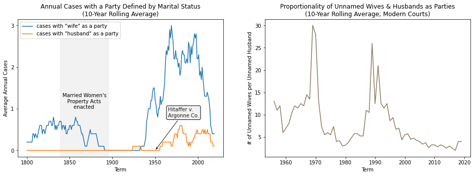
We’ve continued to use et ux. and et vir. in case names up to the present day, with wives consistently going unnamed in cases at a much higher rate than husbands. Variants of et ux. appear in party names at a rate roughly 3 to 5 times that of the variants of et vir. over ten year periods since $2000$.

Leaving a party unnamed on its own case strikes me as among the most effective ways of marginalizing someone through legal procedure. It effectively blocks their participation in legal discourse, seemingly serving as one of the last vestiges of coverture, the common law doctrine that effectively meant a woman’s legal and property rights were transferred to her husband when married. Without her name included in the case, a married woman’s legal contributions to societal progress are also obfuscated in the official record, replaced by a reminder of gender dynamics that should have never existed but at least died generations ago.

And this doesn’t even get into issues of representation for genderqueer married couples, etc.

Why in the world is this term still in use? While Google didn’t turn up any relevant discussion of the term online beyond brief definitions, the Wikipedia entry for et uxor I linked to earlier cites a short but informative article in Legal Affairs by Kristin Collins. Collins lays out the case against et ux. much more eloquently than I’ve done here and covers how problematic the term is more expansively.

Interestingly, she also identifies its merits, observing that its relationship with women’s rights is at least more nuanced than I would have imagined. While arguably denying married women due process, until the Married Women’s Property Acts of 1839, mentioning a woman as an “ux” in a legal document or deed indicated that she had rights to a property (or a portion thereof) if her husband died before her. A century later, the nation’s courts re-examined their case law and legislation regarding loss of consortium following the landmark Hitaffer v. Argonne Co. case in the D.C. Circuit, which recognized a wife’s right to recover damages over a loss of consortium, a right long held by husbands but only recently granted to wives.⁵ With this newfound right to action, “et ux.” began to signal that a woman was filing suit over loss of consortium. While it still seems far more problematic than not, “et ux.” now at very least flags particular legal issues at play in these cases.

In any event, I tend to favor identifying humans by name rather than reducing them to their genders or relationships to the nearest land-owning man. It seems to me that avoiding dehumanizing other people is probably a Best Practice™ in any Definitive Guide to Being a Satisfactory Human. Hopefully the U.S. courts someday agree with this radical idea.

So now that you’ve heard me speaking from up on this soapbox for a bit, you’re probably wondering how all of this connects back to inconsistencies among caseNames. Earlier we made sure to only consider cases with “et” or “and” followed by “uxor”, “ux”, or “wife”. Let’s broaden our search to see what other wives and husbands crop up.

fig, axes = plt.subplots(1, 2, figsize=(16, 5))

axes[0].axvspan(1827.5, 1868.5, color=(0.95, 0.95, 0.95));
axes[0].annotate('The "wife of"\nBoom', (1802.5, 3.0),
                 bbox={'boxstyle': 'round', 'fc': (.99, .99, .99)},
    color=label_font_color,
    zorder=2);

(case_decisions
     .assign(**{'wife': lambda df: df.caseName.str.contains(r'\b(?:ux|uxor|wife|wives)\b', case=False, regex=True),
                'husband': lambda df: df.caseName.str.contains(r'\b(?:vir|husbands?)\b', case=False, regex=True)})
     [['term', 'wife', 'husband']]
     .groupby('term').sum()
     .rolling(10).mean()
     .plot(ax=axes[0], legend=True,
           title='Cases with Names Containing a Variant of "Wife" or "Husband"',
           xlabel='Term', ylabel='Cases (10-Year Average)'))

(case_decisions
     .assign(wives=lambda df: df.caseName.str.count(r'\b(?:ux|uxor|wife|wives)\b', flags=re.IGNORECASE),
             husbands=lambda df: df.caseName.str.count(r'\b(?:vir|husbands?)\b', flags=re.IGNORECASE))
     [['wives', 'husbands']]
     .apply(lambda x: x.rename(x.name).value_counts())
     .fillna(0)
     .plot(kind='bar', logy=True, ax=axes[1],
           title='Cases by # of Appearances of a "Wife" or "Husband" Variant',
           xlabel='Occurrences', ylabel='Cases'));

display(fig, metadata={'filename': f'{ASSETS_DIR}/2021-07-05_Historical_Wife_and_Husband_Variants.png'})
plt.close()

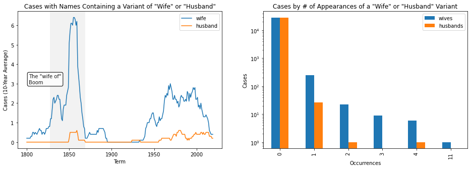
Occurrences of various wife and husband “spellings” appear to follow similar trends to our more restrictive earlier search for variants of et ux. and et vir, which doesn’t seem too surprising. We can also see that the Court has felt less and less of a need to call out marital status in case names in modern times.

unnamed_wives_as_parties = case_decisions.loc[
    case_decisions.caseName.str.contains(r'\b(?:ux|uxor|wife|wives)\b', case=False),
    ['term', 'caseName']
]
unnamed_husbands_as_parties = case_decisions.loc[
    case_decisions.caseName.str.contains(r'\b(?:vir|husbands?)\b', case=False),
    ['term', 'caseName']
]

pd.Series({
    ('Unnamed Wife as Party', 'All Time'): unnamed_wives_as_parties.shape[0],
    ('Unnamed Wife as Party', 'Since 1946'): unnamed_wives_as_parties.term.between(1946, 2021).sum(),
    ('Unnamed Wife as Party', 'Since 2000'): unnamed_wives_as_parties.term.between(2000, 2021).sum(),
    ('Unnamed Husband as Party', 'All Time'): unnamed_husbands_as_parties.shape[0],
    ('Unnamed Husband as Party', 'Since 1946'): unnamed_husbands_as_parties.term.between(1946, 2021).sum(),
    ('Unnamed Husband as Party', 'Since 2000'): unnamed_husbands_as_parties.term.between(2000, 2021).sum()
}).to_frame('Case Counts')

		Case Counts
Unnamed Wife as Party	All Time	290
	Since 1946	130
	Since 2000	17
Unnamed Husband as Party	All Time	28
	Since 1946	21
	Since 2000	6

The annual number of cases containing mention of a “wife”, for instance, is more than halved when moving from 1946–1999 cases to cases occurring in the new millenium. Maybe this can provide some solace for us when noting that, over its entire history, the Court has found a need to call out gender and marital status for women almost ten times more frequently than it has for men.

Wait, no. I said I was stepping down from the soapbox. Back to the data wrangling. How do these $290$ wifely cases break down? You might guess that you’d only see “et ux.” and “and wife” among these case names, but you’d be wrong.

case_decisions[
    case_decisions.caseName.str.contains(r'\b(?:and wife\b|et ux\.)', case=False)
].caseName.size

178

You could tack on “his wife”, and this moves you closer to $290$ but not close enough.

case_decisions[
    case_decisions.caseName.str.contains(r'\b(?:and wife\b|et ux\.|his wife\b)', case=False)
].caseName.size

267

Beyond these, there is a dash of "& wife"s,

case_decisions[
    case_decisions.caseName.str.contains(r'& wife\b', case=False)
].caseName.size

8

a pinch of period-less "et ux"s,

case_decisions[
    case_decisions.caseName.str.contains(r'\bet ux$\b', case=False)
].caseName.size

4

and even one zany "et wife" from the early days of the Court!⁶

case_decisions[
    case_decisions.caseName.str.contains(r'\bet wife\b', case=False)
].caseName.size

1

As you can see, the Court has a knack for butchering language, and we still have ten cases unaccounted for! Of these, nine adopt one of the many strange case naming conventions of the 1800s, exhibited with gusto in the timeless classic Antoine Michoud, Joseph Marie Girod, Gabriel Montamat, Felix Grima, Jean B. Dejan, Aine, Denis Prieur, Charles Claiborne, Mandeville Marigny, Madam E. Grima, Widow Sabatier, A. Fournier, E. Mazureau, E. Rivolet, Claude Gurlie, the Mayor of the City of New Orleans, the Treasurer of the Charity Hospital, and the Catholic Orphan’s Asylum, Appellants, v. Peronne Bernardine Girod, Widow of J. P. H. Pargoud, Residing at Aberville, in the Duchy of Savoy, Rosalie Girod, Widow of Philip Adam, Residing at Faverges, in the Duchy of Savoy, Acting for Themselves and in Behalf of Their Coheirs of Claude Fran Ois Girod, to Wit, Louis Joseph Poidebard, Fran Ois S. Poidebard, Denis P. Poidebard, Widow of P. Nicoud; Jacqueline Poidebard, Wife of Marie Rivolet; Claudine Poidebard, Widow of P. F. Poidebard; and M. R. Poidebard, Wife of Anthelme Vallier, and Also of Fran Ois Quetand, Jean M. F. Quetand, Marie J. Quetand, Wife of J. M. Avit; Fran Oise Quetand, Wife of J. A. Allard; Marie R. Quetand, Marie B. Quetand; Also of J. F. Girod, Jeanne P. Girod, Wife of Clement Odonino, F. Clementine Girod, Wife of P. F. Pernoise, and Jean Michel Girod, Defendants.

with pd.option_context('display.max_colwidth', 1000):
    display(
        case_decisions.loc[
            case_decisions.caseName.str.contains(r'\bwife of\b', case=False),
            ['term', 'caseName']
        ]
    )

	term	caseName
736	1823	HUGH WALLACE WORMLEY, THOMAS STRODE, RICHARD VEITCH, DAVID CASTLEMAN, AND CHARLES M'CORMICK, APPELLANTS, v. MARY WORMLEY, WIFE OF HUGH WALLACE WORMLEY, BY GEORGE F. STROTHER, HER NEXT FRIEND, AND JOHN S. WORMLEY, MARY W. WORMLEY, JANE B. WORMLEY, AND ANNE B. WORMLEY, INFANT CHILDREN OF THE SAID MARY AND HUGH WALLACE, BY THE SAID STROTHER, THEIR NEXT FRIEND, RESPONDENTS
1665	1845	JOHN LANE AND SARAH C. LANE, WIFE OF THE SAID JOHN, AND ELIZABETH IRION, AN INFANT UNDER TWENTY-ONE YEARS, WHO SUES BY JOHN LANE HER NEXT FRIEND, COMPLAINANTS AND APPELLANTS, v. JOHN W. VICK, SARGEANT S. PRENTISS et al., DEFENDANTS
1736	1846	ANTOINE MICHOUD, JOSEPH MARIE GIROD, GABRIEL MONTAMAT, FELIX GRIMA, JEAN B. DEJAN, AINE, DENIS PRIEUR, CHARLES CLAIBORNE, MANDEVILLE MARIGNY, MADAM E. GRIMA, WIDOW SABATIER, A. FOURNIER, E. MAZUREAU, E. RIVOLET, CLAUDE GURLIE, THE MAYOR OF THE CITY OF NEW ORLEANS, THE TREASURER OF THE CHARITY HOSPITAL, AND THE CATHOLIC ORPHAN'S ASYLUM, APPELLANTS, v. PERONNE BERNARDINE GIROD, WIDOW OF J. P. H. PARGOUD, RESIDING AT ABERVILLE, IN THE DUCHY OF SAVOY, ROSALIE GIROD, WIDOW OF PHILIP ADAM, RESIDING AT FAVERGES, IN THE DUCHY OF SAVOY, ACTING FOR THEMSELVES AND IN BEHALF OF THEIR COHEIRS OF CLAUDE FRANCOIS GIROD, TO WIT, LOUIS JOSEPH POIDEBARD, FRANCOIS S. POIDEBARD, DENIS P. POIDEBARD, WIDOW OF P. NICOUD; JACQUELINE POIDEBARD, WIFE OF MARIE RIVOLET; CLAUDINE POIDEBARD, WIDOW OF P. F. POIDEBARD; AND M. R. POIDEBARD, WIFE OF ANTHELME VALLIER, AND ALSO OF FRANCOIS QUETAND, JEAN M. F. QUETAND, MARIE J. QUETAND, WIFE OF J. M. AVIT; FRANCOISE QUETAND, WIFE OF J. A. ALLARD; MARIE R. QUETAND, MAR...
1754	1847	THE UNITED STATES, APPELLANT, v. JOSEPH LAWTON, EXECUTOR OF CHARLES LAWTON, MARTHA POLLARD, HANNAH MARIA KERSHAW WIFE OF JAMES KERSHAW, et al.
1800	1848	SAMUEL L. FORGAY AND ELIZA ANN FOGARTY, WIFE OF E. W. WELLS, APPELLANTS, v. FRANCIS B. CONRAD, ASSIGNEE IN BANKRUPTCY OF THOMAS BANKS
1996	1850	THE UNITED STATES, APPELLANTS, v. SARAH TURNER, THE WIFE OF JARED D. TYLER, WHO IS AUTHORIZED AND ASSISTED HEREIN BY HER SAID HUSBAND; ELIZA TURNER, WIFE OF JOHN A. QUITMAN, WHO IS IN LIKE MANNER AUTHORIZED AND ASSISTED BY HER SAID HUSBAND; HENRY TURNER, AND GEORGE W. TURNER, HEIRS AND LEGAL REPRESENTATIVES OF HENRY TURNER, DECEASED
2103	1851	ALEXANDER H. WEEMS, PLAINTIFF IN ERROR, v. ANN GEORGE, CONELLY GEORGE, ROSE ANN GEORGE, WIFE OF JOHN STEEN, MARY ANN GEORGE, WIFE OF THOMAS CONN, NANCY GEORGE, WIFE OF JAMES GILMOUR, MARGARET GEORGE, WIFE OF WILLIAM MILLER, JOHN STEEN, THOMAS
2154	1852	ELIJAH PEALE, TRUSTEE OF THE AGRICULTURAL BANK OF MISSISSIPPI, PLAINTIFF IN ERROR, v. MARTHA PHIPPS, AND MARY BOWERS, WIFE OF CHARLES RICE
2348	1855	LOUIS CURTIS, BENJAMIN CURTIS, JOHN L. HUBBARD, JAMES D. B. CURTIS, AND HENRY A. BOORAINE, PLAINTIFFS IN ERROR, v. MADAME THERESE PETITPAIN, WIFE OF VICTOR FESTE, AND MANDERVILLE MARIGNY, LATE UNITED STATES MARSHAL FOR THE EASTERN DISTRICT OF

The old-timey “wife of So-and-So” language is born and dies during the 1800s. I haven’t looked into it in any detail, but a reading of the majority opinions in a few of these cases suggests that “Sue Shmoe, wife of Joe Shmoe” is used to flag that Sue is a party to a case, with or without Joe, when Sue is engaging in a property dispute or otherwise exercising her legal rights in relation to a third party. Again, this is just speculation on my part and should be taken with a huge pile of salt.

Last but not least we have one new case containing "the wife" from around the turn of the twentieth century with appellant “Michaela Leonarda Almonester, the wife separated from bed and board of Joseph Xavier Delfau de Pontalba”:

display_inline(
    case_decisions[
        case_decisions.caseName.str.contains(r'\b(?:the wife)\b', case=False)
    ].caseName
)

	caseName
1902	MICHAELA LEONARDA ALMONESTER, THE WIFE SEPARATED FROM BED AND BOARD OF JOSEPH XAVIER DELFAU DE PONTALBA, PLAINTIFF IN ERROR, v. JOSEPH KENTON
1996	THE UNITED STATES, APPELLANTS, v. SARAH TURNER, THE WIFE OF JARED D. TYLER, WHO IS AUTHORIZED AND ASSISTED HEREIN BY HER SAID HUSBAND; ELIZA TURNER, WIFE OF JOHN A. QUITMAN, WHO IS IN LIKE MANNER AUTHORIZED AND ASSISTED BY HER SAID HUSBAND; HENRY TURNER, AND GEORGE W. TURNER, HEIRS AND LEGAL REPRESENTATIVES OF HENRY TURNER, DECEASED

(Note the second case from 1996 was already accounted for in the "wife of" query.)

Just in the seemingly simple example of et ux., we see half a dozen variations on spelling and punctuation, variations that ebb and flow with case naming conventions through the Court’s history. To normalize these values while sticking faithfully to the spirit of the conventions laid out in the SCDB’s documentation could require a careful reading of volumes of the Lawyers’ Edition up to 1946 and Westlaw reports from then on.⁷ I’m all for deep diving into new data sources, but that would require quite a large investment of time, energy, and potentially pocket change for very little gain. Accordingly I’m going to assume they’re of the intended format for the time being and leave any manipulations to when (if ever) I’m engineering features for a model related to these names.

A Cap on Case Names?

These caseNames also exhibit the following issues with long values in the legacy dataset:

• There doesn’t appear to be a consistent convention on how many parties to include prior to an “et al.”.
• The case names do not align with modern case citation conventions.
• Citation styles are varied and often opt for being as verbose as possible.
• caseNames also appear to be capped at $1000$ characters in length.
• The last two effects combine to result in the truncation we saw earlier in a novella of a case name from 1846 and a similar case name from 1850.

with pd.option_context('display.max_colwidth', 1000):
    display(
        case_decisions.loc[
            case_decisions.caseName.str.len() == case_decisions.caseName.str.len().max(),
            ['term', 'caseName']
        ]
    )

	term	caseName
1736	1846	ANTOINE MICHOUD, JOSEPH MARIE GIROD, GABRIEL MONTAMAT, FELIX GRIMA, JEAN B. DEJAN, AINE, DENIS PRIEUR, CHARLES CLAIBORNE, MANDEVILLE MARIGNY, MADAM E. GRIMA, WIDOW SABATIER, A. FOURNIER, E. MAZUREAU, E. RIVOLET, CLAUDE GURLIE, THE MAYOR OF THE CITY OF NEW ORLEANS, THE TREASURER OF THE CHARITY HOSPITAL, AND THE CATHOLIC ORPHAN'S ASYLUM, APPELLANTS, v. PERONNE BERNARDINE GIROD, WIDOW OF J. P. H. PARGOUD, RESIDING AT ABERVILLE, IN THE DUCHY OF SAVOY, ROSALIE GIROD, WIDOW OF PHILIP ADAM, RESIDING AT FAVERGES, IN THE DUCHY OF SAVOY, ACTING FOR THEMSELVES AND IN BEHALF OF THEIR COHEIRS OF CLAUDE FRANCOIS GIROD, TO WIT, LOUIS JOSEPH POIDEBARD, FRANCOIS S. POIDEBARD, DENIS P. POIDEBARD, WIDOW OF P. NICOUD; JACQUELINE POIDEBARD, WIFE OF MARIE RIVOLET; CLAUDINE POIDEBARD, WIDOW OF P. F. POIDEBARD; AND M. R. POIDEBARD, WIFE OF ANTHELME VALLIER, AND ALSO OF FRANCOIS QUETAND, JEAN M. F. QUETAND, MARIE J. QUETAND, WIFE OF J. M. AVIT; FRANCOISE QUETAND, WIFE OF J. A. ALLARD; MARIE R. QUETAND, MAR...
1868	1850	JOHN DOE, LESSEE OF JACOB CHEESMAN, PETER CHEESMAN AND SARAH, HIS WIFE, BEERSHEBA PARKER, WARD PEARCE, JOHN CLARK AND MARGARET, HIS WIFE, ANN JACKSON, WILLIAM JACKSON, SEWARD JACKSON, AND MARY JACKSON, -- WATSON AND SARAH, HIS WIFE (LATE SARAH PEARCE), WILLIAM PEARCE, WARD PEARCE, MIRABA EDWARDS, JAMES EDWARDS, RICHARD PEARCE, WILLIAM, JAMES, AND MARGARET PEARCE, THOMAS MORRIS AND MARY, HIS WIFE (LATE MARY PEARCE), ELIZABETH POWELL (LATE ELIZABETH PEARCE), JACOB WILLIAMS AND ELIZABETH WILLIAMS, SARAH SMALLWOOD, DEBORAH BRYANT, GEORGE L. HOOD AND LETITIA, HIS WIFE, IN HER RIGHT, JOSEPH SMALLWOOD, JOSEPH HURFF, JANE TURNER, JOHN BROWN AND MARY, HIS WIFE, IN HER RIGHT, WILLIAM SMALLWOOD, ISAAC HURFF AND ELIZABETH, HIS WIFE, IN HER RIGHT, RICHARD SHARP AND MARIAM, HIS WIFE, IN HER RIGHT, RANDALL NICHOLSON AND DRUSELLA, HIS WIFE, IN HER RIGHT, JACOB MATTISON AND JEMIMA, HIS WIFE, IN HER RIGHT, JOSEPH NICHOLSON AND MARIAM, HIS WIFE, IN HER RIGHT, THOMAS PEARCE, AND MATTHEW PEARCE, (ALL C...

• Some values appear to be cut off due to data entry errors like the relatively short string "LOUIS CURTIS, BENJAMIN CURTIS, JOHN L. HUBBARD, JAMES D. B. CURTIS, AND HENRY A. BOORAINE, PLAINTIFFS IN ERROR, v. MADAME THERESE PETITPAIN, WIFE OF VICTOR FESTE, AND MANDERVILLE MARIGNY, LATE UNITED STATES MARSHAL FOR THE EASTERN DISTRICT OF", which is $242$ characters in length. This could also be due to some other systemic issue like older, lower character limits in the SCDB’s storage system or in one of their data sources. There’s also a blip in the distribution of case name lengths from the 1800s at around the $240$ character mark that lends credence to the suggestion of a systemic issue.

subplot_width = 9
fig, axes = plt.subplots(1, 2, figsize=(2 * subplot_width, (3 / 5) * subplot_width),
                         sharex=True, sharey=True)
axes[0] = (case_decisions
        .loc[lambda df: df.term.between(1800, 1899), ['caseName', 'term']]
        .assign(
            case_name_length=lambda df: df.caseName.str.len()
        )
        .loc[:,#lambda df: df.case_name_length.between(1, 250),
             'case_name_length']
        .pipe(
            sns.histplot,
            ax=axes[0],
            log_scale=True
        ))
axes[0].set_title('Case Name Lengths in the 1800s')

label_font_color = (0.1, 0.1, 0.1)
axes[0].annotate('The $240$ Blip', xy=(230, 100), xytext=(100, 400), xycoords='data',
            arrowprops={'arrowstyle': 'simple', 'color': arrow_color},
            bbox={'boxstyle': 'round', 'fc': annotation_fill_color},
            color=label_font_color,
            fontsize=14)

axes[1] = (case_decisions
        .loc[lambda df: df.term.between(1946, 2020),
             ['caseName', 'term']]
        .assign(
            case_name_length=lambda df: df.caseName.str.len()
        )
        .loc[:, 'case_name_length']
        .pipe(
            sns.histplot,
            ax=axes[1]
        ))
axes[1].set_title('Modern Case Name Lengths');

display(fig, metadata={'filename': f'{ASSETS_DIR}/2021-07-05_Case_Name_Length_Distributions.png'})
plt.close()

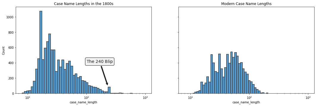
Whatever their origins, these truncation issues are easily fixed after we get identify the offending cases. While this task can be challenging in general⁸, we know the shorter of the two truncation points occurs around $240$ characters, and cases with names of this length are rare in the dataset.

So rare are long case names that I can manually identify and correct truncated case names containing $240$ or more characters all by my lonesome without losing my mind. I’ve decided to go down the manual route and leave a more sophisticated solution that identifies shorter truncated case names for another day. (More accurately, I’ve left such a solution for someone who has more of a need for it than me!) We begin by collecting all case names with lengths at least $240$ characters (with some wiggle room), the shorter of the two lengths around which truncation occurs.

print(
    'Case names containing at least 230 characters:',
    case_decisions.loc[(case_decisions.caseName.str.len() >= 230), 'caseName']
                  .shape[0]
)

Case names containing at least 230 characters: 132

(I used a minimum case name length of $230$ to provide a bit of a buffer for where truncation begins, based on the histogram.) We can also immediately rule out any cases that end in one of the party descriptors “defendant”, “respondent”, and “appellee” or their plural forms, since these are almost always the last words in case names in the SCDB when present. This cuts down the number of cases to review by $11$.

print(
    'Remaining Cases to Review:',
    case_decisions.loc[
        (case_decisions.caseName.str.len() >= 230)
        & ~case_decisions.caseName.str.contains(r'(?:respondent|defendant|appellee)s?\.?$',
                                                regex=True, case=False),
        'caseName'
    ].shape[0]
)

Remaining Cases to Review: 121

Sifting through these cases, I found $67$ were likely truncated, most of them clearly so.

truncated_case_ids = [
    '1828-022', '1828-051', '1834-022', '1836-022', '1836-030', '1836-051',
    '1839-030', '1843-010', '1843-019', '1843-020', '1843-031', '1844-027',
    '1846-039', '1847-022', '1847-031', '1848-006', '1848-023', '1849-009',
    '1849-011', '1849-015', '1849-024', '1850-004', '1850-010', '1850-039',
    '1850-043', '1850-117', '1850-122', '1850-127', '1851-010', '1851-013',
    '1851-027', '1851-029', '1851-043', '1851-059', '1851-065', '1851-066',
    '1851-077', '1851-081', '1852-003', '1852-033', '1852-044', '1852-045',
    '1852-046', '1853-008', '1853-026', '1853-050', '1853-078', '1854-007',
    '1854-048', '1855-011', '1855-013', '1855-015', '1855-067', '1855-071',
    '1855-081', '1856-024', '1856-031', '1857-035', '1857-055', '1857-056',
    '1859-045', '1859-090', '1860-014', '1860-040', '1860-044', '1873-160',
    '1916-105'
]

truncated_case_indices = (
    case_decisions.caseId.isin(truncated_case_ids)
                  .pipe(lambda is_truncated: is_truncated.index[is_truncated])
)

display_inline(
    case_decisions.loc[
        case_decisions.caseId.isin(truncated_case_ids[:5]),
        'caseName'
    ]
)

	caseName
916	JAMES ELLIOTT THE YOUNGER, BENJAMIN ELLIOTT, ANDERSON TAYLOR, REUBEN PATER, PATSEY ELLIOTT, AND WILFORD LEPELL, VS. THE LESSEE OF WILLIAM PEIRSOL, LYDIA PEIRSOL, ANN NORTH, JANE NORTH, SOPHIA NORTH, ELIZABETH F. P. NORTH, AND WILLIAM NORTH, DE
945	JAMES D'WOLF, JUNIOR, PLAINTIFF IN ERROR, VS. DAVID JACQUES RABAUD, JEAN PHILIPPE FREDERICK RABAUD, ALPHONSE MARC RABAUD, ALIENS, AND SUBJECTS OF THE KING OF FRANCE, AND ANDREW E. BELKNAP, A CITIZEN OF THE STATE OF MASSACHUSETTS, DEFENDANTS I
1209	WILLIAM YEATON, THOMAS VOWELL, JUN., WILLIAM BRENT, AUGUSTINE NEWTON AND DAVID RECKETS, ADMINISTRATORS OF WILLIAM NEWTON, AND OTHERS, APPELLANTS v. DAVID LENOX AND OTHERS, AND ELIZABETH WATSON AND ROBERT J. TAYLOR, ADMINISTRATRIX AND ADMINISTR
1312	BURTIS RINGO, JAMES ELLIOTT, JOHN COLLINS, JOHN ELLIOTT, JAMES LAWRENCE, THOMAS WATSON, ATHEY ROWE, GEORGE MUSE, SEN. AND GEORGE MUSE, JUN., APPELLANTS v. CHARLES BINNS AND ELIJAH HIXON, STEPHEN HIXON, NOAH HIXON, JOHN HIXON, WILLIAM HIXON AN
1320	THOMAS LELAND AND CYNTHIA B. LELAND HIS WIFE, LEMUEL HASTINGS, GEORGE CARLTON AND ELIZABETH WAITE CARLTON HIS WIFE, WILLIAM JONES HASTINGS, JONATHAN JENKS HASTINGS, LAMBERT HASTINGS, JOEL HASTINGS, HUBBARD HASTINGS AND HARRIET MARIA HASTINGS,

With the offending cases identified, this is a great opportunity to take advantage of the aforementioned Caselaw Access Project’s API to recover the full case names. The CAP API will most likely recognize the SCDB ID of each of these cases.⁹

def fetch_cap_case_data(scdb_id, auth_token=os.getenv('CAP_AUTH_TOKEN')):
    request_kwargs = {}
    if auth_token is not None:
        request_kwargs['headers'] = {'Authorization': f'Token {auth_token}'}

    results = requests.get(
        f'https://api.case.law/v1/cases/?cite=SCDB{scdb_id}',
        **request_kwargs
    ).json()['results']

    if results:
        return results[0] if len(results) == 1 else results


truncated_case_cap_data = pd.Series({
    index: fetch_cap_case_data(scdb_id)
    for index, scdb_id in zip(truncated_case_indices, truncated_case_ids)
})

assert truncated_case_cap_data.map(bool).all()

untruncated_case_names = truncated_case_cap_data.map(lambda cap_data: cap_data['name'])

We’re not out of the woods yet; there’s still an outside chance that the CAP provided the name for a different case. We’ll use RapidFuzz to verify that the corrected case names are sufficiently similar¹⁰.

assert all(
    fuzz.partial_token_set_ratio(scdb_name, cap_name, processor=True) > 95
    for scdb_name, cap_name in zip(
        case_decisions.loc[truncated_case_indices, 'caseName'],
        untruncated_case_names
    )
)

I feel safe replacing the SCDB case names with those from the CAP after the RapidFuzz sanity check. Before doing so, however, we’ll transform the CAP case names into the normal SCDB format. All of these cases have two named opposing parties, which makes life easy.

corrected_case_names = untruncated_case_names.str.upper().str.replace(r'\bV(?:ERSU)?S?\b', 'v', regex=True)

assert (corrected_case_names.str.count(r'\bv\b') >= 1).all()

case_decisions.loc[truncated_case_indices, 'caseName'] = corrected_case_names

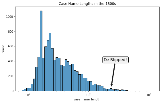
So how did we do? Did we get rid of the cap¹¹? It does look like we’ve all but rid ourselves of the $240$ blip and smoothed out the long tail of case name lengths.

subplot_width = 9
fig, axes = plt.subplots(1, 1, figsize=(subplot_width, (3 / 5) * subplot_width),
                         sharex=True, sharey=True, squeeze=False)
axes[0][0] = (case_decisions
    .loc[lambda df: df.term.between(1800, 1899), ['caseName', 'term']]
    .pipe(
        lambda df: df.caseName.str.len().rename('case_name_length')
    )
    .pipe(
        sns.histplot,
        ax=axes[0][0],
        log_scale=True
    ))
axes[0][0].set_title('Case Name Lengths in the 1800s')

label_font_color = (0.1, 0.1, 0.1)
axes[0][0].annotate(
    'De-Blipped!', xy=(240, 50), xytext=(180, 400), xycoords='data',
    arrowprops={'arrowstyle': 'simple', 'color': arrow_color},
    bbox={'boxstyle': 'round', 'fc': annotation_fill_color},
    color=label_font_color,
    fontsize=14);

display(fig, metadata={'filename': f'{ASSETS_DIR}/2021-07-05_Case_Name_Lengths_in_1800s_De-Blipped.png'})
plt.close()

Case Name Lengths over Time

After digging a little deeper we can also see some issues which may or may not have anything to do with how records were entered into the SCDB. Notably, the Court¹² went hog wild with its mid-nineteenth century case names.

DARK_PURPLE = (0.451271, 0.125132, 0.507198, 1.0)


def length_distribution_by_period(df, value_column, time_column, period_years):
    length_column = f'{value_column}_length'
    period_column = f'{time_column}_period'
    return (
        df[[value_column, time_column]]
            .assign(**{
                length_column: df[value_column].str.len().astype(int),
                period_column: df[time_column].map(lambda term: pd.Period(term, freq=f'{period_years}Y'))
            })
            .pipe(
                lambda df: pd.get_dummies(df[length_column])
                             .cumsum()
                             .set_index(df[period_column]))
            .groupby(period_column)
            .last()
            .diff(period_years)
            .dropna()
            .pipe(lambda df: df.div(df.sum(axis='columns'), axis='index')))


@contextmanager
def mpl_backend_context(new_backend):
    original_backend = mpl.get_backend()
    importlib.reload(mpl)
    mpl.use(new_backend)
    importlib.reload(plt)
    try:
        yield
    finally:
        mpl.use(original_backend)
        importlib.reload(plt)


def distribution_animation_init():
    ax.set_xlim(x_min, x_max)
    ax.set_xlabel('Case Name Length')
    
    ax.set_ylim(y_min, y_max)
    ax.set_ylabel('Proportion of Cases')

    ax.set_frame_on(False)
    return plt.plot([], [])


def frame_artists_and_metadata(df, static_end_frames=60):
    frame_artists = []
    for index_and_column in enumerate(df.columns):
        yield frame_artists, *index_and_column
    for _ in range(static_end_frames):
        yield frame_artists, *index_and_column


def update_distribution_frame(frame_artists_and_metadata, alpha_decay_factor=0.5, colormap=lambda _: DARK_PURPLE):
    frame_artists, frame_index, frame_year = frame_artists_and_metadata

    if not frame_artists:
        frame_artists.append(plt.text(0.87 * x_max, 0.97 * y_max, '', fontsize=12))
    frame_artists[0].set_text(f'{(pd.Timestamp(str(frame_year)) - period_years).year}–{frame_year}')

    for earlier_distribution in frame_artists[1:]:
        earlier_distribution.set_alpha(alpha_decay_factor * earlier_distribution.get_alpha())
    distribution = plt.plot(
        name_length_distribution_per_quarter_century.index,
        name_length_distribution_per_quarter_century[str(frame_year)],
        color=colormap(0.25 + frame_index / (2 * number_of_years)),
        alpha=1
    )[0]
    frame_artists.append(distribution)
    return frame_artists


def embed_local_video(path: Path):
    encoded_video = base64.b64encode(path.read_bytes())
    return HTML(
        data=f'''
        <video width="640" height="480" autoplay loop controls>
            <source src="data:video/mp4;base64,{encoded_video.decode('ascii')}" type="video/mp4" />
        </video>
        '''
    )


period_years = pd.DateOffset(years=25)
name_length_distribution_per_quarter_century = case_decisions.pipe(
    length_distribution_by_period, 'caseName', 'term', period_years.years
).T


with mpl_backend_context('Agg'):
    fig, ax = plt.subplots(figsize=(9, 6));
    fig.suptitle(f'Case Name Lengths\n(Distribution over {period_years.years}-Year Periods)', fontsize=14)

    number_of_years = name_length_distribution_per_quarter_century.shape[1]

    x_min, x_max = 0, 300
    y_min, y_max = 0, 1.02 * name_length_distribution_per_quarter_century.to_numpy().max()

    static_end_frames = 45
    name_length_distribution_per_quarter_century_animation = mpl_animation.FuncAnimation(
        fig,
        update_distribution_frame,
        frames=frame_artists_and_metadata(
            name_length_distribution_per_quarter_century,
            static_end_frames=static_end_frames
        ),
        interval=60,
        save_count=name_length_distribution_per_quarter_century.shape[1] + static_end_frames,
        blit=True,
        repeat=True,
        repeat_delay=10000,
        init_func=distribution_animation_init
    );

    name_length_distribution_per_quarter_century_animation.save(
        f'{ASSETS_DIR}/2021-07-05_Case_Name_Length_Distribution_per_Quarter_Century.mp4',
        bitrate=-1, dpi=300
    );


embed_local_video(ASSETS_DIR / '2021-07-05_Case_Name_Length_Distribution_per_Quarter_Century.mp4')

This animated, rolling distribution illustrates the temporality of case name lengths over time. Case names started small, exploded into novellas in the early- to mid-1800s, returned to being terse before the Warren court of the mid-1940s, and have been relatively stable since. I have no idea what mix of differences between Lawyers’ Edition and Westlaw naming conventions, inconsistent data entry, changing Court norms, and changing case subject matter contributed to these trends, but they’re there and surprisingly pronounced.

It might be interesting to look at how case naming conventions evolve over time using a more consistent data source in the future. For now I choose to imagine this data as reflecting a passive-aggressive, centuries-long war between factions of justices. A war reflecting a Court dialectic on data curation, in which each new generation of justices raises a reactionary banner in response to its predecessor’s brevity or verbosity.

Is this realistic? Absolutely not. Is it funny? I think so. Is this a sign I’ve spent too much time looking at case names in this dataset? Almost surely. Let’s move on.

Appendix: From Case Names to Parties

While we’re not aiming to do any feature engineering in this series, a question that naturally presents itself when processing case names is how to extract petitioners and respondents (both individually and as groups) into their own variables. This is slightly more involved that what you might guess, since (a) there are plenty of single party case names to contend with like In re John Doe and (b) both the separator used between petitioners and respondents and the capitalization of party names are both inconsistent. The right way to go about this is (1) sanitize the data some, getting rid of unexpected characters and normalizing punctuation and formatting; (2) cook up a simple set of regular expressions that covers all of the expected case name formats; and (3) manually address inevitable stragglers. As an illustration of how awful your life will be without step (1), the following code identifies parties in all but 0.3% of cases without any initial data cleansing.

named_party = r'(?:[-–_.,;:\'’* &()\[\]/%$#0-9A-Z]|et al\.)+'

case_parties_cert = fr'(?P<probable_petitioner>{named_party}) ?\b(?:VERSUS\b|v\.?) ?(?P<probable_respondent>{named_party})'
case_parties_in_re = r'(?:IN THE )?MATTER OF (?P<subject_matter>.+)|(?:(?i)in re) (?P<latin_subject_matter>.+)'
case_parties_ex_parte = r'ex parte (?P<ex_partay1>.+)|(?P<ex_partay2>.+), ex parte'
case_parties_boat = (
    '(?P<some_boat>'
        'THE [-.\sA-Z]+'
        '(?:'
            '.+ '
            '(?:CLAIMANTS?|LIBELLANTS?|MASTER)'
        ')?'
        '[.,\s]*'
        '(?:\([A-Z\s]+\'S\s+CLAIM[.,)]?)?'
    ')'
)

parties_pattern = f'^{"|".join([case_parties_cert, case_parties_in_re, case_parties_ex_parte, case_parties_boat])}$'

case_parties = (case_decisions.caseName.str.extract(parties_pattern)
                              .assign(ex_party=lambda df: df.ex_partay1.fillna(df.ex_partay2),
                                      re_party=lambda df: df.subject_matter.fillna(df.latin_subject_matter))
                              .drop(columns=['ex_partay1', 'ex_partay2',
                                             'subject_matter', 'latin_subject_matter']))

unmatched_case_names = case_decisions.loc[
    case_parties.isna().all(axis='columns'),
    ['term', 'caseName']
]

display(
    case_parties.notna().sum(axis='index')
)

print('\nCases with Unidentified Parties:', unmatched_case_names.shape[0], end='\n\n')

with pd.option_context('display.max_colwidth', 2000):
    display_inline(
        unmatched_case_names.head(),
        unmatched_case_names.tail()
    )

probable_petitioner    27952
probable_respondent    27952
some_boat                449
ex_party                 214
re_party                 182
dtype: int64



Cases with Unidentified Parties: 78

	term	caseName
5	1792	HAYBURN'S CASE
448	1815	SHIP SOCIETE, MARTINSON, MASTER
637	1820	LA AMISTAD DE RUES. -- ALMIRAL, LIBELLANT
773	1824	TWO HUNDRED CHESTS OF TEA, SMITH, CLAIMANT
807	1825	SIXTY PIPES OF BRANDY. KENNEDY & MAITLAND, CLAIMANTS

	term	caseName
15005	1918	THE SCOW 6-S
15024	1918	ARIZONA EMPLOYERS' LIABILITY CASES
16992	1927	THE MALCOLM BAXTER, JR.
17997	1934	ATCHISON, TOPEKA & SANTA FE RAILWAY CO. et al.
18043	1934	GORDON, SECRETARY OF BANKING, et al.

While these are in no way the worst set of regular expressions I’ve ever seen in code, they’re made unnecessarily complex since we did not sanitize the data. Even with more self-documenting code and color commentary, I wouldn’t look forward to returning to this kludge next year to extend it to support more cases. The regex is also incomplete in its functionality. I brain dumped the above code as an example, so it fails to pick up a smattering of case names including the always popular <random inanimate object> v. United States collection. There are also 32 case names that look like CYRIL FIGGIS v. JOE v. SCHMOE or JOE v. SCHMOE v. CYRIL FIGGIS in the SCDB, presumably due to a half-baked find and replace in the dataset’s past. These are unlikely to fare well under this search scheme.

That said, similar code, in conjunction with some automated and manual cleansing, could quickly yield a nicely extracted set of parties organized by party type and the broad categories into which each case falls. And since this isn’t a huge dataset that’s getting updated rapidly by many contributors, it’s probably a decent means of extracting party names without too much effort.

assert case_parties[['probable_petitioner', 'probable_respondent']].notna().sum(axis='columns').isin({0, 2}).all()

assert case_parties[
    case_parties[['probable_petitioner', 'probable_respondent']].notna().sum(axis='columns') == 0
].notna().sum(axis='columns').isin({0, 1}).all()

case_parties.head()

	probable_petitioner	probable_respondent	some_boat	ex_party	re_party
0	WEST, PLS. IN ERR.	BARNES. et al.	<NA>	<NA>	<NA>
1	VANSTOPHORST et al.	THE STATE OF MARYLAND	<NA>	<NA>	<NA>
2	OSWALD, ADMINISTRATOR,	THE STATE OF NEW-YORK	<NA>	<NA>	<NA>
3	OSWALD, ADMINISTRATOR,	THE STATE OF NEW-YORK	<NA>	<NA>	<NA>
4	THE STATE OF GEORGIA	BRAILSFORD, et al.	<NA>	<NA>	<NA>

I’ll leave logically consolidating these five columns into two and splitting out lists of party members into their own columns as exercises for the reader.

Updating DVC … Elsewhere

One of the goals of this series was to demonstrate simple DVC pipelines by example. In my first post, I began building a simple DVC pipeline for tracking our changes to each SCDB dataset. The scripts defining the pipeline were generated within the post’s notebook for illustration purposes, although I pointed out at the time that I do not recommend vomiting notebook code into scripts and calling the result “production code”. (Or worse still, just running notebooks as production code directly.) My opinions on if and when to use notebooks, notebooks as an anti-pattern, best practices when developing ML workflows, etc. would require more lines than I’m willing to give them here. I’m open to write a follow-up on the subject if there’s interest. Because of these opinions, a desire to avoid maintainability issues, and an interest in sharing these datasets, I’ve decided to avoid writing any updates to the DVC pipeline in these posts. I don’t want to appear to endorse productionizing code from notebooks, even if I would only appear to be doing so to folks who aren’t actually reading my prose.

Instead, I’ve released an updated version of the pipeline and the derived datasets on DAGsHub and mirrored its contents sans data to GitHub. Going forward, all of the changes I make to the SCDB datasets in these notebooks will be reflected in updates to this pipeline, and updated datasets will be downloadable from the DAGsHub repository. These repositories will be the best places to see how the pipeline evolves over time.

If you’re new to DAGsHub you should check it out. It’s basically a diet version of GitHub that’s DVC-aware and can also host data artifacts from your DVC pipelines. This DVC awareness is exposed through the UI in a variety of ways, the most immediately obvious of which being its pretty, interactive visualizations of your data pipeline(s):

(There is, unfortunately, no clear way to embed an interactive pipeline diagram into another webpage at the time of writing this, hence the above screenshot.)

Next Steps

And there we have it—another post and a tidier SCDB dataset. This was by far the lengthiest of the three posts so far, and hats off to you if you made it through all of my rambling! This has blown up into a larger effort than I originally intended, mostly due to my interest in using it as an excuse to experiment with writing long-form blog posts. I admit that I’m getting antsy to move on to related projects I have in the hopper or, really, anything other than basic cleansing, feature by feature, of SCDB datasets. Nevertheless, I’ll see this series through, although perhaps in a more succinct style. We’ve just covered the “Identification Variables” within the SCDB as well as one of the “Background Variables” (caseName). In future posts we’ll move on to other Background Variables followed by Chronological, Substantive, Outcome, and Voting & Opinion Variables. From what I’ve seen while working through most of this data preparation work in advance, there isn’t as much to discuss when cleansing the majority of these variables compared to caseNames, so I imagine I can get away with a higher features per post score in the future.

And then, of course, I have a few different posts planned that are based on SCDB and CAP data sources that anyone still reading will really enjoy. These might include an excursion into language modeling; answering the question posed by Opening Arguments that I alluded to in the first post; and different approaches to analyzing, visualizing, and predicting the voting behavior of Supreme Court justices. If you’re enjoying the series, have ideas for future work, would like to collaborate, or spotted some typos, don’t hesitate to reach out.

Appendix: Trivia

Here are a couple odds and ends about the stickier parts of the United States that didn’t fit well in the main post.

What’s the beef between Texas and Oklahoma?

In the last post we resisted the urge to look into why Oklahoma and Texas had such an unneighborly relationship last century. The reason, in case anyone else was wondering, isn’t terribly exciting or surprising—boundary disputes:

oklahoma_or_texas = r'(?:STATE OF )?(?:OKLAHOMA|TEXAS)'

oklahoma_v_texases = case_decisions.loc[
    case_decisions.caseName.str.contains(
        fr'{oklahoma_or_texas} v\.? {oklahoma_or_texas}', case=False
    ),
    ['usCite', 'dateDecision', 'caseName', 'issue']
].sort_values(by='dateDecision').reset_index(drop=True)

display_inline(
    (10 * (oklahoma_v_texases.dateDecision.dt.year // 10)).value_counts(sort=False).to_frame('Decade'),
    oklahoma_v_texases.issue.value_counts().to_frame('Issue')
)

	Decade
1920	28
1930	1
1980	1

	Issue
state boundary dispute	21
state property dispute	7
misc. interstate conflict	2

I wouldn’t be surprised if all of the cases from the 1920s and 1930s, and possibly the lone case from the 1980s, should all be classified as state boundary disputes, but I haven’t mustered the willpower to read through nine cases that I can only imagine are chock-full of metes and bounds. I have to look out for my own quality of life before embarking on that sort of deep dive. While we’re here, note the cornucopia of punctuation choices and party descriptions that come up even when cases seem this straightforward to name.

oklahoma_v_texases.caseName.value_counts().to_frame('Cases')

	Cases
STATE OF OKLAHOMA v. STATE OF TEXAS. UNITED STATES, INTERVENER	15
STATE OF OKLAHOMA v. STATE OF TEXAS, UNITED STATES, INTERVENER	7
STATE OF OKLAHOMA v. STATE OF TEXAS; UNITED STATES, INTERVENER	2
STATE OF OKLAHOMA v. STATE OF TEXAS.; UNITED STATES, INTERVENER	1
OKLAHOMA v. TEXAS, UNITED STATES, INTERVENER	1
OKLAHOMA v. TEXAS	1
OKLAHOMA v. TEXAS; UNITED STATES, INTERVENOR	1
OKLAHOMA v. TEXAS; UNITED STATES, INTERVENER	1
TEXAS v. OKLAHOMA	1

Yes, it would be simple to standardize the punctuation and naming here, but this would just be the tip of the iceberg, as I hope the above post illustrates. Adopting a standard set of conventions across all case names would be a larger endeavor than I’m willing to commit to, since I don’t have any projects planned that would get significantly more use out of the refined names.

How Unique are Case Names?

Notwithstanding the impression you might have after seeing so many Oklahoma v. Texas cases above, most cases in the SCDB have unique names.

def unique_ratio(series):
    return (series.value_counts()
                  .pipe(lambda name_counts: (name_counts == 1).sum()
                                                / len(name_counts)))


legacy_cases = case_decisions[case_decisions.term < 1946]
modern_cases = case_decisions[case_decisions.term >= 1946]

print(
    'Share of Legacy Cases with Unique Names:',
    round(unique_ratio(legacy_cases.caseName), 4)
)

print(
    'Share of Modern Cases with Unique Names:',
    round(unique_ratio(modern_cases.caseName), 4)
)

print(
    'Share of All Cases with Unique Names:',
    round(unique_ratio(case_decisions.caseName), 4)
)

Share of Legacy Cases with Unique Names: 0.964
Share of Modern Cases with Unique Names: 0.9772
Share of All Cases with Unique Names: 0.9661

1. I’m so sorry you had to read that. ↩

2. Note that I’ve excluded case citations here that contain characters other than Arabic numerals in their page numbers, resulting in these numbers being close but imperfect approximations. ↩

3. For the sake of your mental health, dear reader, I have done my absolute best to avoid BCE and CE puns here. I reserve the right to do so at a later date. ↩

4. I had originally assumed that Spaeth considered the Warren Court the start of the modern era due to its departure from traditions of its judicially and politically conservative predecessors, with the Vinson Court laying tracks for some of its more groundbreaking rulings. That doesn’t appear to be the case, however, given Spaeth’s “Prefatory Note” in the SCDB documentation describes legacy cases as “those decided between 1791 and the Court’s acquisition of discretionary jurisdiction as a result of the Judges’ Bill of 1925”. While I have done some digging into the history of the Judiciary Act of 1925 and its consequences, I have yet to find a persuasive argument for why (of if) the start of the Vinson court should be considered the dawn of the modern era of the court rather than, say, one of the intervening years between the passage of the Judges’ Bill and then. Based on a preliminary analysis of the SCOTUS dockets from these and surrounding terms, the dust begins to settle and the composition of the SCOTUS caseload is on its way to a new normal by 1946, but that term again feels rather arbitrary to me. There are also other structural changes to the Court and its administration in the 1930s that could play into this decision, but again I’m only going off of a small number of statements in the SCDB documentation and related materials. If you are able to shed more light on this division, I’d love to hear from you. ↩

5. For further reading on loss of consortium, I found this summary helpful. It’s also interesting to see contemporary perspectives on the Hitaffer v. Argonne Co. ruling and how they shift over time. ↩

6. See Calder et Wife v. Bull et Wife. ↩

7. Beyond a bunch of manual relabeling, a saner way to standardize these case names would involve comparing them to the case names coming from another reliable source for case metadata. We do something similar to detruncate case names below, using a combination of the CAP API (defined below) for alternative case names and RapidFuzz for fuzzy string comparison. ↩

8. If we suspected that truncation was also occurring for shorter case names, we could attempt to flag and fix the shortened names in two different ways. The first way will probably be obvious after reading this section—replace a case name with the corresponding name provided by the CAP whenever the former is sufficiently similar (in some fuzzy metric) to the latter. This approach is the simplest, but it’s not without issues, not the least of which is that it’s replacing case names in the SCDB with analogs from official U.S. Reports. This would result in a departure from the SCDB documentation, which I’m trying to avoid. There are also errors in some CAP case names, and some cases in the SCDB are difficult or impossible to find in the CAP. If you don’t have a research account for the CAP, this will also be painfully slow, since you’re limited to $500$ requests per day through their API and can’t access their bulk downloads. I don’t consider this a real issue, since (I have researcher access, and) you can request researcher access for free through their website, but it’s still a barrier to getting started if you’re new to the CAP. These issues can be partially remedied by also pulling in case information from the CourtListener API, but there will still probably be gaps in the case information we can pull.

   The other approach I mentioned is to analyze the SCDB case names themselves and attempt to flag names that appear truncated. This more intrinsic approach can replace or supplement the one above and can be broken down into two phases. First the easy part: identifying which cases end in a truncated word. We could get to a pretty decent solution by filtering out case names whose last words (after being lower cased and stripped of punctuation) are

   • common legalese stop words (al. from et al. for instance);
   • surnames (e.g., using Philippe Rémy’s name-dataset package;
   • correctly spelled words in English, Spanish, German, and French (using a package like pyspellchecker;
   • common abbreviations;
   • city names using something like Simple Maps’s World Cities and U.S. Cities datasets; or
   • (the last words in) state and territory names.

   This is conceptually one big dictionary lookup for the last word in each case name—not that you’d implement it that way (I hope). It’s straightforward to implement in Pandas and can probably sift out 90+% of cases without any additional effort. With more work you can get this sort of process to leave you with almost exclusively records ending in truncated words without dropping any on the floor.

   For the cases that were filtered out in the previous step, we can then move on to phase two: identifying untruncated words that are unlikely to appear at the end of a case name. This is where quite a bit of finesse could be necessary, and the general task seems impossible. For instance, some of the case names we’re detruncating here end with a party’s last name and look perfectly valid; they are just lacking additional listed parties or some kind of description. Without a third-party case name to compare to, it would be next to impossible to detect that kind of truncation. Still, we might have some success flagging cases with, for instance,

   • last words that are odd parts of speech (prepositions, for instance);
   • last words that are first names; and
   • unusual terminal $n$-grams (after replacing rare words like names with common tokens).

   ↩

9. If the CAP API doesn’t find a case when searching by SCDB ID, we can then try to look up the case using one of its other citations. That said, I’ve found that the CAP is unlikely to find a case by any of its other citations if it fails to recognize its SCDB ID. In this rare set of circumstances, using another service like CourtListener can usually dig up the case. ↩

10. Roughly, this means long substrings exist in both case names that are mostly comprised of the same sets of words after preprocessing (lowercasing and removing special characters and excess whitespace). ↩

11. Will calling this process “decapitation” lose me any readers? ↩

12. Or a tired SCDB intern, or a ten year old making pennies per week in the Dickensian offices of West back in the 1800s. Who’s to say? Well, I imagine the good folks at the SCDB are, but why waste their time when I can speculate on the internet? ↩