The Great SCOTUS Data Wrangle, Part 2: Missing Values from on High
Happy Belated New Year! I’m back, vaccinated, and eager to drudge through old Supreme Court opinions!
In my
previous post, I began prepping data from the
Supreme Court Database
for use in answering a question posed on the
Opening Arguments podcast. I
began by retrieving and reading an SPSS distribution of the
database into a Pandas
DataFrame. I then tidied up its data types, flagged missing values, and
fixed an errant record by reading the corresponding SCOTUS and
lower court opinions. I concluded the basic data wrangling by
writing the resulting dataset to a new feather file, before
capturing this process as a simple data pipeline using
DVC.
This post will pick up where our last one left off with more data wrangling, or at least preparing for more data wrangling. What’s left on this front mostly boils down to handling missing values where possible, which is simultaneously a less and more interesting problem than usual for this data. On the one hand, only the most basic, run-of-the-mill techniques prove useful for automated imputation. On the other, this is one of the rare moments where we have a real world dataset in which the entire population is completely known to us! Because I am looking at past Supreme Court opinions, which are public record and readily attainable, I could, in theory, correct every missing value in the dataset by reading through every Supreme Court opinion (and probably many lower court opinions) in U.S. history. Of course, this would take an eternity, involve contacting the SCDB curators whenever I stumbled on ambiguous values where their internal conventions mattered, and probably require I either get a law degree or farm out some analysis to a lawyer. We’ll see how far I can get without bringing in bigger guns.
My experiment in long-form, notebook-driven data wrangling in blog
form has quickly become less a blog post and more a blog series.
In this the second installment of said series, I’ll be looking
over the remaining variables of interest in the SCDB and getting a
sense of how their missing values are distributed, demonstrating
my favorite parts of the
missingno
package along the way. I’ll leave the actual imputation work for
follow up posts.
I’ve attempted to strike a healthy balance in what follows, doing original research to fill in missing information when the amount of reading required is relatively small (a couple dozen opinions I need to read in full or at most a couple hundred I need to skim) but mostly sticking to automated methods. I thought that this would have the added benefit of keeping the post to a slightly more reasonable length, but this has blown up thanks to a mix of the ambition of the original plan and my compulsion to share some of the oddities I find along the way.
Let’s get to it!
from pathlib import Path
from typing import Mapping, Union

import git
import numpy as np
import matplotlib.pyplot as plt
import missingno as msno
import pandas as pd

REPO_ROOT = Path(git.Repo('.', search_parent_directories=True).working_tree_dir).absolute()
DATA_PATH = REPO_ROOT / 'data'

case_decisions = pd.read_feather(
    DATA_PATH / 'processed' / 'scdb' / 'SCDB_Legacy-and-2020r1_caseCentered_Citation.feather'
)
Remaining Variables of Interest
As I’ve said, there are more columns in this dataset than we need for the analysis I’m planning. We’ll save a huge amount of time by restricting our cleaning tasks to just the columns that are likely to be of some use in this project. At times, we’ll cut down on work even further by ignoring the “legacy” cases from terms prior to 1946, since they largely won’t play into our analysis and disproportionately contribute to data inconsistency problems.
The SCDB codebook breaks down the variables in this database into six distinct categories: identification, background, chronological, substantive, outcome, and voting and opinion. To keep things a bit easier to read and navigate, I plan to follow the same categorization scheme in follow-up posts.
identification_variables_of_interest = ['caseId']

background_variables_of_interest = [
    'caseName',
    'petitioner',
    'petitionerState',
    'respondent',
    'respondentState',
    'jurisdiction',
    'certReason'
]

chronological_variables_of_interest = ['chief', 'naturalCourt']

substantive_variables_of_interest = [
    'issue',
    'issueArea',
    'lawType',
    'lawSupp',
    'lawMinor',
    'decisionDirection',
    'decisionDirectionDissent',
    'authorityDecision1',
    'authorityDecision2'
]

outcome_variables_of_interest = [
    'decisionType',
    'declarationUncon',
    'caseDisposition',
    'caseDispositionUnusual',
    'partyWinning',
    'precedentAlteration'
]

voting_and_opinion_variables_of_interest = ['majOpinWriter', 'voteUnclear']

categorical_interests = [
    *identification_variables_of_interest,
    *background_variables_of_interest,
    *chronological_variables_of_interest,
    *substantive_variables_of_interest,
    *outcome_variables_of_interest,
    *voting_and_opinion_variables_of_interest
]
A Bird’s Eye View of Missing Values
As a well-curated set of mostly categorical features, the SCDB has
few fields with room for data consistency issues. All but one of
its non-numeric, non-datetime columns are restricted to a small,
documented set of values. The remaining
caseName
variable is unstructured and contains inconsistencies we’ll
discuss in a later post.
By far the biggest issue with this dataset is null values. The SCDB’s documentation makes clear that this is due in part to many variables being sparsely encoded, but we’ll also find a fair share of these values are genuinely missing.
Before proceeding any further, however, we should normalize our
nulls. For reasons I haven’t looked into (presumably having to do
with our conversion of this data from SPSS files), missing
categorical values are expressed several different ways, none of
which are bona fide
NaNs.
case_decisions.isna().to_numpy().sum()
0
For the sake of exposition, I catalogued the dataset’s assortment
of null value flags in advance so that we can map them all to
np.nans
here. (For the curious Data Science Dojo attendee out there, I
didn’t do anything special to find these values. I just catalogued
them when looking at
value_counts for each variable.)
null_values = {np.nan, None, 'nan', 'NA', 'NULL', '', 'MISSING_VALUE'}

case_decisions = (case_decisions
        .mask(case_decisions.isin(null_values), np.nan)
        .pipe(lambda df: pd.concat([
            df.select_dtypes(exclude='category'),
            df.select_dtypes(include='category')
              .apply(lambda categorical: categorical.cat.remove_unused_categories())
        ], axis='columns')))

pd.concat(
    [
        case_decisions[categorical_interests].describe().T,
        pd.Series({
            column: len(case_decisions[case_decisions[column].isna()])
            for column in categorical_interests
        }, name='null_value_counts').to_frame()
    ],
    axis='columns'
)
| count | unique | top | freq | null_value_counts | |
|---|---|---|---|---|---|
| caseId | 28891 | 28891 | 1918-055 | 1 | 0 |
| caseName | 28885 | 27655 | STATE OF OKLAHOMA v. STATE OF TEXAS. UNITED ST... | 15 | 6 |
| petitioner | 28889 | 273 | United States | 2509 | 2 |
| petitionerState | 3730 | 57 | United States | 296 | 25161 |
| respondent | 28887 | 259 | United States | 3118 | 4 |
| respondentState | 6297 | 58 | United States | 667 | 22594 |
| jurisdiction | 28889 | 14 | cert | 10355 | 2 |
| certReason | 28803 | 13 | no cert | 18577 | 88 |
| chief | 28891 | 17 | Fuller | 4986 | 0 |
| naturalCourt | 28891 | 106 | Waite 6 | 1591 | 0 |
| issue | 28776 | 277 | liability, nongovernmental | 1403 | 115 |
| issueArea | 28776 | 14 | Economic Activity | 8376 | 115 |
| lawType | 27557 | 8 | No Legal Provision | 10767 | 1334 |
| lawSupp | 27557 | 187 | No Legal Provision | 10806 | 1334 |
| lawMinor | 5130 | 2978 | tax law | 808 | 23761 |
| decisionDirection | 28798 | 3 | liberal | 13037 | 93 |
| decisionDirectionDissent | 28658 | 2 | dissent in opp. direction | 28572 | 233 |
| authorityDecision1 | 28774 | 7 | statutory construction | 10512 | 117 |
| authorityDecision2 | 4191 | 7 | statutory construction | 1522 | 24700 |
| decisionType | 28890 | 7 | opinion of the court | 26273 | 1 |
| declarationUncon | 28890 | 4 | no unconstitutional | 27519 | 1 |
| caseDisposition | 28635 | 11 | affirmed | 13226 | 256 |
| caseDispositionUnusual | 28889 | 2 | no unusual disposition | 28671 | 2 |
| partyWinning | 28874 | 3 | petitioner lost | 15894 | 17 |
| precedentAlteration | 28890 | 2 | precedent unaltered | 28627 | 1 |
| majOpinWriter | 26664 | 110 | MRWaite | 1000 | 2227 |
| voteUnclear | 28887 | 2 | vote clearly specified | 28786 | 4 |
Excluding the fact that the states of
Oklahoma and Texas have
apparently sued each other at least $15$ times, the most striking
thing about this data is that the only categorical
variables under study without missing values are the
caseId
primary key of this version of the SCDB, the chief justice
indicator
chief,
and the
naturalCourt
tracker. Two of these,
caseId
and
naturalCourt, are presumably auto-generated, while
chief is
the easiest column in the database to fill in. So no,
unfortunately, we don’t live in a perfect world, and even a
dataset as meticulously curated as the SCDB has its flaws.
That said, the second and more important thing that jumps out at
me is the distribution of those
null_value_counts. Nearly half of the $27$ features have fewer than $20$ null
values. Assuming there is some relationship between when some of
these features are missing (that is, assuming they are
missing not at random), manual correction of these variables is a possibility.
(Aside: It’s fun to be working with data for once where manual correction is feasible. This tends to be very difficult in industry—especially when working alone—due to a number of factors including the immensity of the data being studied and potentially having no access to the ground truth. Here the only real potential problems are statistical concerns like introducing bias in a subjective field, which I plan on treating gently.)
We can also see that the closely-related fields
issue
and
issueArea
contain the exact same number of
null_value_counts, as do
lawType
and
lawSupp.
Interrelations between “missingnesses” of these features can
simplify imputation by enabling us to impute one’s values using
the other’s and by speeding up the manual correction process.
Manually correcting the remaining $50\%$ of features is well beyond the scope of what I’m willing to do for this article, but it’s worth noting that many of these features contain more than $1000$ missing values. I’m hoping that at very least these features are among those that are sparsely encoded.
The picture is also much less grim in the modern dataset, but there are still large swaths of missing values to contend with.
is_modern_decision = case_decisions.term >= 1946

pd.concat(
    [
        case_decisions.loc[is_modern_decision, categorical_interests].describe().T,
        pd.Series({
            column: len(case_decisions[is_modern_decision & case_decisions[column].isna()])
            for column in categorical_interests
        }, name='null_value_counts').to_frame()
    ],
    axis='columns'
)
| count | unique | top | freq | null_value_counts | |
|---|---|---|---|---|---|
| caseId | 9030 | 9030 | 2012-054 | 1 | 0 |
| caseName | 9030 | 8784 | UNITED STATES v. CALIFORNIA | 8 | 0 |
| petitioner | 9030 | 263 | State | 906 | 0 |
| petitionerState | 1835 | 56 | California | 218 | 7195 |
| respondent | 9029 | 244 | State | 1410 | 1 |
| respondentState | 2524 | 55 | California | 240 | 6506 |
| jurisdiction | 9029 | 11 | cert | 7313 | 1 |
| certReason | 8944 | 13 | no reason given | 3213 | 86 |
| chief | 9030 | 5 | Burger | 2809 | 0 |
| naturalCourt | 9030 | 34 | Rehnquist 7 | 973 | 0 |
| issue | 8971 | 266 | search and seizure (gen.) | 251 | 59 |
| issueArea | 8971 | 14 | Criminal Procedure | 2040 | 59 |
| lawType | 7772 | 8 | Fed. Statute | 2742 | 1258 |
| lawSupp | 7772 | 176 | Infrequent litigate (Code) | 1558 | 1258 |
| lawMinor | 1553 | 940 | 28 U.S.C. § 1257 | 24 | 7477 |
| decisionDirection | 8992 | 3 | liberal | 4534 | 38 |
| decisionDirectionDissent | 8853 | 2 | dissent in opp. direction | 8773 | 177 |
| authorityDecision1 | 8973 | 7 | statutory construction | 3851 | 57 |
| authorityDecision2 | 1455 | 7 | statutory construction | 527 | 7575 |
| decisionType | 9030 | 6 | opinion of the court | 7052 | 0 |
| declarationUncon | 9030 | 4 | no unconstitutional | 8375 | 0 |
| caseDisposition | 8897 | 11 | affirmed | 2692 | 133 |
| caseDispositionUnusual | 9030 | 2 | no unusual disposition | 8862 | 0 |
| partyWinning | 9014 | 3 | petitioner won | 5765 | 16 |
| precedentAlteration | 9030 | 2 | precedent unaltered | 8845 | 0 |
| majOpinWriter | 7300 | 38 | BRWhite | 475 | 1730 |
| voteUnclear | 9029 | 2 | vote clearly specified | 8940 | 1 |
We’ll turn to
missingno
to round out our high-level picture of missing values in the
dataset.
legacy_case_count = case_decisions.shape[0] - is_modern_decision.sum()

msno.matrix(
    case_decisions[categorical_interests],
    labels=True
);
plt.plot([-0.5, len(categorical_interests) - 0.5], 2 * [legacy_case_count], 'r');
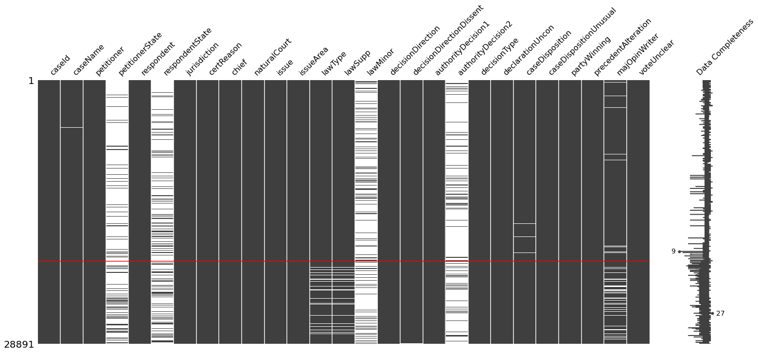
If you’re new to
missingno, the above is a
figure-ground
depiction of the completeness of each variable in the dataset,
where the figure and ground represent the presence and absence of
variable values throughout the dataset, respectively. I’ve also
added a red line at the boundary between the legacy and modern
subsets of the data. This type of “nullity1
matrix” can be a great tool for quickly gaining understanding
about what data is missing from a dataset, how missing values are
related within and between variables, and speculate on data source
issues that could be contributing factors.
Unfortunately the above example is not the most useful, but we can
still glean a few pieces of information about connections. One
thing that jumps out is a possible relationship between missing
values in the
majOpinWriter,
lawType,
and
lawSupp
columns beginning in the modern dataset. My guess is that this
arises due to a growing number of per curiam opinions in
modern cases.
per_curiam_decision_types = {
    'per curiam (oral)',
    'per curiam (no oral)',
    'equally divided vote'
}

per_curiam_rate_legacy = (
    case_decisions[(case_decisions.term < 1946)]
        .pipe(lambda df: df.decisionType.isin(per_curiam_decision_types).sum() / df.shape[0])
)
per_curiam_rate_modern = (
    case_decisions[(case_decisions.term >= 1946)]
        .pipe(lambda df: df.decisionType.isin(per_curiam_decision_types).sum() / df.shape[0])
)

print('Rate of Per Curiam Decisions Pre-Vinson Court (1791–1945):', per_curiam_rate_legacy)
print('Rate of Per Curiam Decisions Pre-Vinson Court (1946–2019):', per_curiam_rate_modern)
Rate of Per Curiam Decisions Pre-Vinson Court (1791–1945): 0.027541412819092694
Rate of Per Curiam Decisions Pre-Vinson Court (1946–2019): 0.18427464008859357
Yep, a nearly 7-fold increase in per curiam opinions from
the modern Court. A per curiam opinion is typically
anonymous—only insofar as they are unsigned—and brief, typically
sparing words for the Court’s decision with no discussion of the
case. Accordingly, these opinions also are likely to be missing
the information used by the SCDB authors to provide
lawType
and
lawSupp
values.2
The nullities of the
lawType
and
lawSupp
fields also appear to be very well
correlated[^nullity-correlation]. Beyond these connections, I’m
not getting too much new information from this visual for our
dataset.
For a more detailed picture, we can generate a nullity correlation heatmap for these features.
msno.heatmap(
    case_decisions[categorical_interests],
    labels=True
).set_title('Nullity Correlation Heatmap', fontdict={'fontsize': 24});
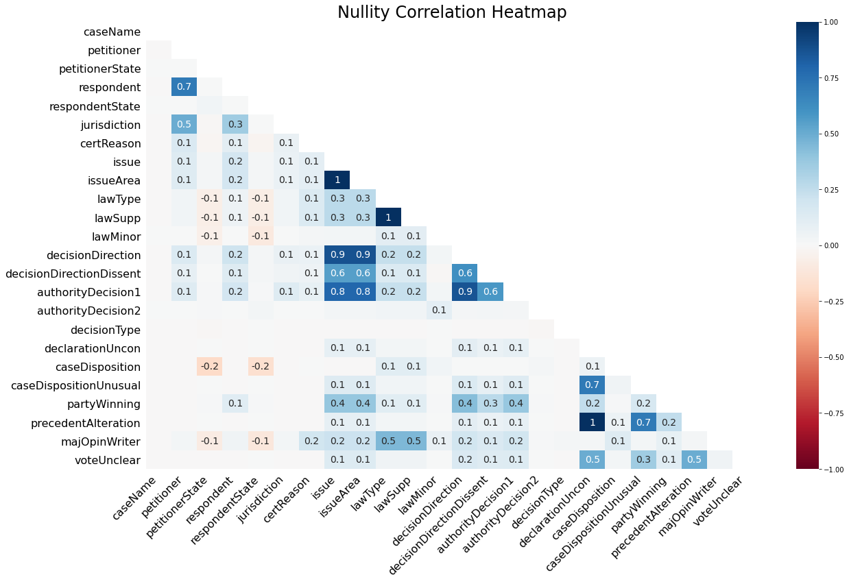
Takeaways
I hope you can see why this is usually the visualization I jump to
when using
missingno. While perhaps less pretty than the figure-ground plot, we get a
much better sense of the correlations between missing values
across variables in the SCDB. To highlight a few that are of note,
-
Missing values in
issueandissueArea,lawTypeandlawSupp, andprecedentAlterationanddeclarationUnconare all perfectly positively correlated, which is to say these pairs are missing from the dataset in the same records. -
Both
decisionDirectionandauthorityDecision1nullities are strongly correlated withissueandissueArea. Indeed, theissue*variables are missing in $90$ of the $93$ cases that are also missing adecisionDirectionand $92$ of the $117$ cases missing anauthorityDecision1. I’ve found that the SCDB documentation is solid enough that this close a relationship is usually well-documented, and true to form, the documentation ofissueArea,decisionDirection, andauthorityDecision1make clear that the decision processes governing their values are functions of theissuevariable, among others. If anything, it would be interesting to take a look at the handful of cases whereissueis missing but with adecisionDirectionorauthorityDecision1to confirm they fall into a fork in the decision process that doesn’t depend onissue. -
There is a fairly high correlation of $0.7$ between
petitionerandrespondentnullities. I was confused by this at first, since I would’ve expected missing value indicators for these variables to be very highly, if not perfectly, correlated. (Whatever their source is for a given record, I would expect it to either contain both a petitioner and respondent or neither.)On inspection, however, the lower-than-expected nullity correlation is more illustrative of how deceptive correlations can be when blindly relied on than it is an inconsistent relationship between null values in these columns. Of the $28,891$ cases in the SCDB, four of them are missing
respondents and two are missingpetitioners, and the two cases missingpetitioners are also missingrespondents. In other words,petitionerandrespondentagree in all but two records (over $99.99\%$ of the dataset), with $\mathtt{respondent} = \mathtt{petitioner}$ a perfectly-fit linear model for all but those two outliers.The problem is, then, that missing values are such rare events. A whole $99.99\%$ of the $99.99\%$ of records in which
petitionerandrespondentagree occur at the origin in thepetitionernullity-respondentnullity plane. The remaining four points are equally divided between points $(1, 1)$ and $(0, 1)$ in that plane, which should (and does) impact the correlation. Increasing the number of $(1, 1)$ pairs in the list even slightly should have a large impact on the correlation coefficient. -
There are a large number of moderately correlated nullities,
including those for
lawType,lawSupp, andmajOpinionWriterthat we observed earlier. More than I’m willing to list here! - There don’t appear to be any dichotomous relationships between nullities of different variables, wherein one variable tends to only be present when the other is missing (as would be exhibited by a strong negative correlation between features in the heatmap.)
While they don’t shine light on the missing values in the SCDB,
it’s also worth noting
missingno
rounds out its core offerings with
dendrograms
of your feature nullities. If you haven’t used it, I highly
recommend it!
What’s Next?
In post number 3, we’ll begin cleaning up the IDs and background
variables within the SCDB. That should involve the most complex
(and least useful to clean) variable in the entire dataset:
caseName. You should probably expect to see the triumphant return of DVC
in that post, as well.
Footnotes
-
The “nullity” of a random variable $X$ is just the dummy variable $\chi_{\texttt{NaN}}(X)$, that is, the
NaN-indicator applied to $X$. ↩ -
Quoting from the
lawTypedocumentation:The basic criterion to determine the legal provision(s) is the “summary” in the Lawyers’ Edition. Supplementary is a reference to it in at least one of the numbered holdings in the summary of the United States Reports. This summary, which the Lawyers’ Edition of the U.S. Reports labels “Syllabus By Reporter Of Decisions,” appears in the official Reports immediately after the date of decision and before the main opinion in the case. Where this summary lacks numbered holdings, it is treated as though it has but one number.